感谢 @awesome-xu 同学帮忙整理
矩阵
矩阵是什么
也许各位对矩阵的了解都是从"解方程组"开始的,但实际上矩阵的意义远远不止于此。实际上,矩阵在计算机图形学中永远十分广泛的应用。甚至于说,如果没有矩阵,那么也不会有三维游戏、三维动画之类的艺术形式。
也许你已经猜到了,矩阵能用来描述空间甚至"控制"空间。这么说有点夸张,所以不妨我们从简单的开始理解。
我们先从最简单的列数与行数相等的矩阵——方阵开始理解。
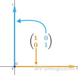
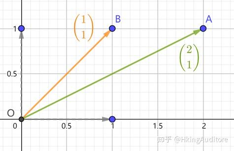
现在有一个
的矩阵
\begin{pmatrix} 1 \\ 2 \\ 3 \\ \end{pmatrix}
,按照我们上一章的说法,它是一个向量。那么现在给出两个
的矩阵
\begin{pmatrix} 1 \\ 0 \\ \end{pmatrix},\begin{pmatrix} 0 \\ 1 \\ \end{pmatrix}
,我们便可以将之理解为表示两个在二维空间中的基向量。
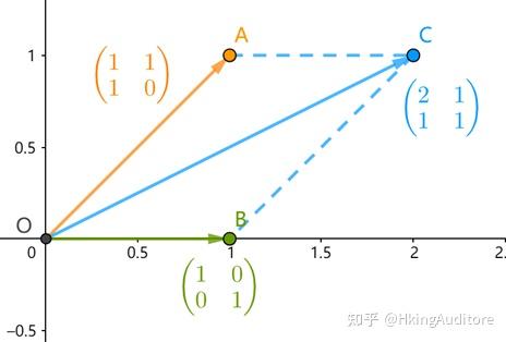
现在我们可以更进一步了:比如尝试将两个向量组合起来写:
\begin{pmatrix} 1 & 0 \\ 0 & 1 \\ \end{pmatrix}\\
现在我们得到了一个
的矩阵,而且我们现在完全可以把它当做一个由两个二维向量构成的向量组,构成成员分别是
\begin{pmatrix} 1 \\ 0 \\ \end{pmatrix},\begin{pmatrix} 0 \\ 1 \\ \end{pmatrix}
。我们称这种对角线元素为1其余元素为0的方阵为单位矩阵(identity matrix)。根据上一章所学,它正好张成了一个十分标准的二维空间:
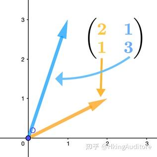
但实际上大多数情况下我们遇到的矩阵并非如此的标准,那么形如
\begin{pmatrix} 2 & 1 \\ 1 & 3 \\ \end{pmatrix}
的矩阵也能如此理解吗?
当然可以,我们可以如此拆分:
这就是一个以
\begin{pmatrix} 2 \\ 1 \\ \end{pmatrix},\begin{pmatrix} 1 \\ 3 \\ \end{pmatrix}
为基向量的二维空间。根据我们在上一章的知识,此时的空间里的"网格线"也会被改变。所以新的空间中应该呈现出下图的模样。
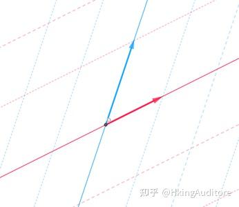
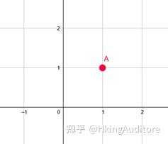
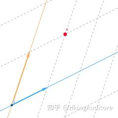
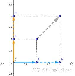
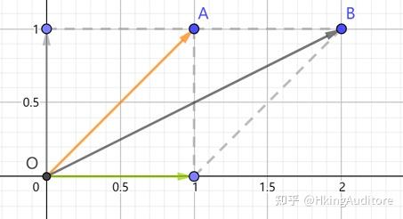
如果我们在原来的
\begin{pmatrix} 1 & 0 \\ 0 & 1 \\ \end{pmatrix}
空间中设定一个点
,那么在新空间这个点A便会随着空间的变换到新的位置。如下面两张图的变化,仿佛是我们把一个空间斜着压了一下,但空间中每个点的相对位置却不会改变。
从
\begin{pmatrix} 1 & 0 \\ 0 & 1 \\ \end{pmatrix}
到
\begin{pmatrix} 2 & 1 \\ 1 & 3 \\ \end{pmatrix}
,虽然同样是张成二维空间,但是它们各自对空间的描述方式的不同的,对此我想给出一种理解方阵的思路:
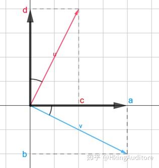
方阵的每一列都代表了单位矩阵中对应列的向量在单位矩阵张成的空间中重新指向的位置。如下图,原来黑色的两条规规矩矩的单位向量纷纷指向了对应的红色、蓝色向量,成为了新的单位向量。矩阵
\begin{pmatrix} a & c \\ b & d \\ \end{pmatrix}
即代表对于
\begin{pmatrix} 1 & 0 \\ 0 & 1 \\ \end{pmatrix}
张成空间,将向量
\begin{pmatrix} 1 \\ 0 \\ \end{pmatrix}
转到
\begin{pmatrix} a \\ b \\ \end{pmatrix}
、将向量
\begin{pmatrix} 0 \\ 1 \\ \end{pmatrix}
转到
\begin{pmatrix} c \\ d \\ \end{pmatrix}
。当然,对于更高维度的空间也是如此。
现在我们知道了矩阵在几何上的意义,但是好像并不能用这套理论完全解释明白所有我们遇到的矩阵。譬如
\begin{pmatrix} 1 & 3 & 5 \\ 2 & 4 & 6 \\ \end{pmatrix}
或
\begin{pmatrix} 1 & 4 \\ 2 & 5 \\ 3 & 6 \\ \end{pmatrix}
这类非方阵,我们该如何在几何上理解它们呢?
不妨先找回我们在上一章中的思路:
\begin{pmatrix} 1 & 3 & 5 \\ 2 & 4 & 6 \\ \end{pmatrix}
就是一个由三个向量组成的向量组,这个向量组张成了一个二维空间,但这毕竟是基于向量组的思路;我们在方阵的理解中引入了对单位矩阵中各单位向量进行变换的思路,所以对于这样一个非方阵,我们是否能找到一个单位矩阵能够巧妙地担负起这个使命?我们不妨先给这个非方阵补0:,把它补成一个方阵:
\begin{pmatrix} 1 & 2 & 3 \\ 4 & 5 & 6 \\ 0 & 0 & 0 \\ \end{pmatrix}\\
因为这三个列向量它们各自本身就是只有
与
分量的向量,因此我们完全可以把它们视作z分量为0的三维向量。于是顺理成章地我们找到了这个矩阵对应的单位矩阵:
\begin{pmatrix} 1 & 0 & 0 \\ 0 & 1 & 0 \\ 0 & 0 & 1 \\ \end{pmatrix}
。
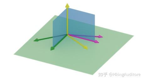
对于这种
的矩阵,我们可以这样理解:如上图,向量
\begin{pmatrix} 0 \\ 0 \\ 1 \\ \end{pmatrix}
被转到了
平面上。也就是图中的垂直于绿色平面的黄色向量被转移到了绿色平面上的黄色向量。转移后的三条向量只能张成一个二维平面空间,因此不妨这么说:一个
的矩阵代表着一个将三维空间变换至二维空间的降维过程。可以进一步推广:任意一个行数小于列数的矩阵,都可以理解为表示一个降维的空间变化。
那如果是对于一个
的矩阵,如
\begin{pmatrix} 1 & 0 \\ 1 & 0 \\ 1 & 1 \\ \end{pmatrix}
,我们该如何理解呢?
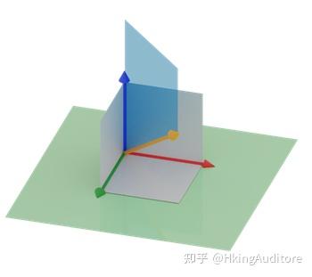
我们可以用同样的思想把它拆分开:
如上图所示,橙色向量即
\begin{pmatrix} 1 \\ 1 \\ 1 \\ \end{pmatrix}
,深蓝色向量即
\begin{pmatrix} 0 \\ 0 \\ 1 \\ \end{pmatrix}
。我们先找到由两个单位向量构成的单位矩阵
\begin{pmatrix} 1 & 0 \\ 0 & 1 \\ \end{pmatrix}
,为了方便后面的理解,我们不妨给这两个向量补充一个
分量,视作
\begin{pmatrix} 1 & 0 \\ 0 & 1 \\ 0 & 0 \\ \end{pmatrix}
,分别对应图中的绿色向量与红色向量。根据之前所述的矩阵变换思路,我们将绿色向量变换到了橙色向量,红色向量变换到了蓝色向量。经过这一番变换,张成的空间从原来的
平面变换到了图中的蓝色平面区域,我们获得了描述
分量的能力,像是进入了三维空间。不过,仔细看的话你会发现,这其实并不是一个真正的三维空间,更准确的说应该是,立在三维世界里的一个平面。对于这种增加了可描述分量但不增加张成空间维数的空间变换,我称之为“名义上的升维"。
我们在前文说过,
个向量最多张成
维空间;而
列的矩阵表示对对应空间中的
条个基向量进行变换,得到了结果自然也是
个向量,所以最多也只能张成
维空间。所以说,对一个空间进行矩阵变换并不会增加原空间的维数。
把我们的结论进行推广,我们发现:一个
的非方阵描述的是一个将
维空间变换至"名义"
维空间的过程。现在叙述这个过程也许会有些难以理解,我们会在之后的学习中详细讲述。
还有一个问题:为什么矩阵是矩阵,向量组是向量组?
其实,两者是本质是相似的。但我通常更喜欢这么看:向量组表示多个向量张成的空间,而矩阵表示将原空间的基向量变换至新的位置得到新的基向量。简单地说:向量组表示空间,矩阵表示变换。
矩阵运算
矩阵数乘
我们在上一章讲过,标量乘法具有缩放的作用。推广开,这在矩阵上也是成立的。
比如我想把一个二维坐标轴放大至两倍,可以这么写:
2 \times \begin{pmatrix} 1 & 0 \\ 0 & 1 \\ \end{pmatrix} = \begin{pmatrix} 2 & 0 \\ 0 & 2 \\ \end{pmatrix}\\
体现到图形上,表现为坐标系中每个点都由原点扩大至原来的两倍:
显然,数乘矩阵就是把矩阵每个元素乘上标量值,得到一个新矩阵。
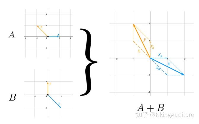
矩阵加法
如果想把两个矩阵的变换效果叠加在一起,就使用矩阵加法吧。矩阵加法就是把两个同型号矩阵,根据元素对应两两相加得到新矩阵,例如:
\begin{pmatrix} 1 & 1 \\ 1 & 0 \\ \end{pmatrix} + \begin{pmatrix} 1 & 0 \\ 0 & 1 \\ \end{pmatrix} = \begin{pmatrix} 2 & 1 \\ 1 & 1 \\ \end{pmatrix}\\
不妨用图解进一步了解其意义:
原标准空间:
矩阵变换
\begin{pmatrix} 1 & 1 \\ 1 & 0 \\ \end{pmatrix}
为:
矩阵变换
\begin{pmatrix} 1 & 0 \\ 0 & 1 \\ \end{pmatrix}
为:
结果变化
\begin{pmatrix} 2 & 1 \\ 1 & 1 \\ \end{pmatrix}
为:
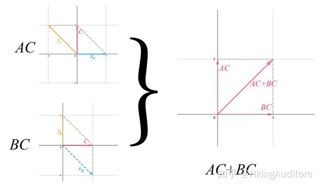
可以用向量加法的原理把得到的变换C拆开进行解释,譬如
\begin{pmatrix} 2 \\ 1 \\ \end{pmatrix}
,其实就是
的第一列向量
\begin{pmatrix} 1 \\ 1 \\ \end{pmatrix}
加上
的第一列向量
\begin{pmatrix} 1 \\ 0 \\ \end{pmatrix}
:
另一个基的运算也同理。
但是需要注意到这样一个问题,矩阵加法中两个相加的矩阵都是基于标准空间解释的。
怎么理解?同样是画图:
标准空间经A变换后,基向量变为了
\begin{pmatrix} 1 \\ 1 \\ \end{pmatrix}
和
\begin{pmatrix} 1 \\ 0 \\ \end{pmatrix}
,在这个新空间中的点
是在图上的点A还是点B呢?
显然是B,只有
\overrightarrow{OB} = 1 \times \begin{pmatrix} 1 \\ 1 \\ \end{pmatrix} + 1 \times \begin{pmatrix} 1 \\ 0 \\ \end{pmatrix}
,而A只是在原来的
\begin{pmatrix} 1 & 0 \\ 0 & 1 \\ \end{pmatrix}
空间中才被解释为
,在新空间里它应被解释为
。
更准确地说,加法中两个矩阵是相对于你为它们坐标命名时所用空间进行解释的。有时你未必会使用常用的
正交空间,而是一些其他空间进行运算。
加法的这一性质使它与矩阵乘法有了区别。
矩阵乘法
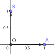
矩阵与向量相乘
矩阵乘法与向量乘法是相通之处的;矩阵处理的是空间变换,而向量便是观察空间变换的绝佳载体。
首先,把这个过程叫做"乘法"确实会让人产生误解,它实际上并不那么像我们想象中的乘法,它更像是把变换应用于目标上。
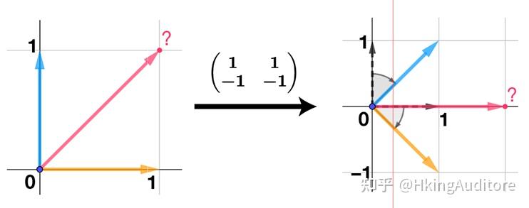
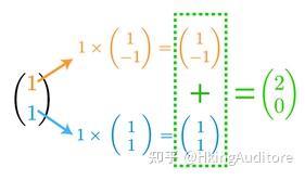
从我们的目标出发吧:假设在一个标准的二维空间中定义了一个向量
\begin{pmatrix} 1 \\ 1 \\ \end{pmatrix}
,然后用矩阵
\begin{pmatrix} 1 & 1 \\ -1 & 1 \end{pmatrix}
对这个空间进行了变换,那么向量
\begin{pmatrix} 1 \\ 1 \end{pmatrix}
会移动到哪里呢?
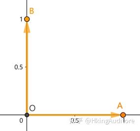
不妨先这样想:我们是如何给出向量的坐标
\begin{pmatrix} 1 \\ 1 \\ \end{pmatrix}
的?在标准空间
\begin{pmatrix} 1 & 0 \\ 0 & 1 \\ \end{pmatrix}
中,取第一个基的一倍,再取第二个基的一倍,将两个向量相加,得
1 \times \begin{pmatrix} 1 \\ 0 \\ \end{pmatrix} + 1 \times \begin{pmatrix} 0 \\ 1 \\ \end{pmatrix} = \begin{pmatrix} 1 \\ 1 \\ \end{pmatrix}
。
这么看来,当我们给出向量坐标时,其实给出的是相对于所选空间所选基下,向量指向位置的解释。因为这是一个相对性的表述,所以我们改变基时,向量的绝对位置就会改变,但它对于新基下的解依旧是不变的。
有个通俗的生活例子可以解释,假设你与你朋友不得不分开乘坐出租车前往某地,当你朋友开动后,你对你的司机说:"用和前面那辆车一样的速度跟着它。"前车的速度就是你的司机判断自身快慢的"基速度",前车如果从60加到70,那你的车速也会从60加到70。在旁人看起来你的车变快了,但是你的司机会说:"我现在的速度依旧是前车一样啊!"
回到矩阵的场合,当我们用“取1个第一个基向量,再取1个第二个基向量,最后把两者相加"来解释
\begin{pmatrix} 1 \\ 1 \\ \end{pmatrix}
,一切都变得简单了。
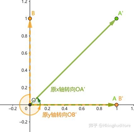
我们知道矩阵变化的一层含义是“变化基向量";在上文所述的空间
\begin{pmatrix} 1 & 1 \\ - 1 & 1 \\ \end{pmatrix}
中,第一个基向量被指定是
\begin{pmatrix} 1 \\ - 1 \\ \end{pmatrix}
,第二个基向量被指定是
\begin{pmatrix} 1 \\ 1 \\ \end{pmatrix}
,那么在这个新空间下,如何解释
\begin{pmatrix} 1 \\ 1 \\ \end{pmatrix}
呢?
在变化基向量后,原来的
\begin{pmatrix} 1 \\ 1 \\ \end{pmatrix}
指向了
\begin{pmatrix} 2 \\ 0 \\ \end{pmatrix}
。当然这个
\begin{pmatrix} 2 \\ 0 \\ \end{pmatrix}
依旧是基于空间
\begin{pmatrix} 1 & 0 \\ 0 & 1 \\ \end{pmatrix}
解释的,可以叫它"绝对位置"。
相信你已经可以给出矩阵乘向量的意义了:用一组新的基处理一个向量,并求这个向量在我们命名时所用基下的位置。或者说:用新的基向量解释向量,再放回原空间表示。
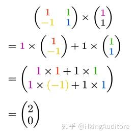
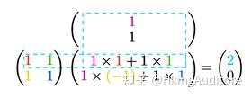
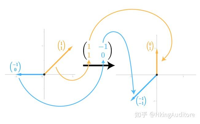
写出计算过程(注意颜色的对应关系):
也就是说:
这正是课本上给出的计算方法!
当然,还有几个问题需要解答:
看看我们的演算过程:"取
倍第1个向量,再取入
倍第2个向量......,再取
倍第
个向量,把它们相加。"因此只有
的矩阵能处理
维的向量,不然无法保证对应关系。
上一节我们知道了:非方阵意味着"名义的"升维与降维,同理,非方阵与向量相乘意味着对原向量进行名义上的维度变换。因为这代表着用高维基表示低维向量。
还有一个棘手的问题:矩阵与向量乘法的左右顺序意味着什么?实际上,所有基于列空间矩阵算式都是从右往左读的,在定义上,这意味着用左边的变化处理右边的式子。具体的含义在下一节可以得到阐述。
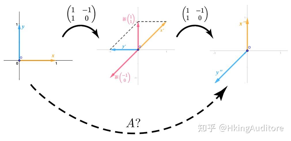
矩阵与矩阵相乘
我们在上一节了解了如何用矩阵去变换一个向量,于是我们很自然地会有这么一个问题:我们是否可以用矩阵去变换另一个矩阵?
我们依旧从一个具体的目标出发:对于一个变换
\begin{pmatrix} 1 & - 1 \\ 1 & 0 \\ \end{pmatrix}
;我想在变换后的空间里将基向量变换至新空间里的
\begin{pmatrix} 1 & - 1 \\ 1 & 0 \\ \end{pmatrix}
,求这个变换的最终形式
。
我们相信,这个效果叠加的变换一定可以写成一种以刚开始进行变换时用的基描述的形式。也就是说,一定有一个矩阵可以一步达到两次变换的结果。
你也许会想到矩阵加法,但务必注意:加法时参照基总是以初始状态为准的,而与变换的过程无关。你可以试着用
\begin{pmatrix} 1 & - 1 \\ 1 & 0 \\ \end{pmatrix} + \begin{pmatrix} 1 & - 1 \\ 1 & 0 \\ \end{pmatrix} = \begin{pmatrix} 2 & - 2 \\ 2 & 0 \\ \end{pmatrix}
,用这个变换根本得不到图中的
空间。
那我们可以试着换一个思路,既然矩阵每一列都是新的基向量的指向,那为什么我们不把它拆分开,再运用我们上一节学到的矩阵向量乘法,得到它在新空间中的位置,那样我们不就得到了两次变换后基向量的最终位置了吗?
按照这个思路,我们将
\begin{pmatrix} 1 & - 1 \\ 1 & 0 \\ \end{pmatrix}
分开为
\begin{pmatrix} 1 \\ 1 \\ \end{pmatrix}
和
\begin{pmatrix} - 1 \\ 0 \\ \end{pmatrix}
,根据矩阵与向量相乘的思路,在
\begin{pmatrix} 1 & - 1 \\ 1 & 0 \\ \end{pmatrix}
空间中,我们取它的
\begin{pmatrix} 1 \\ 1 \\ \end{pmatrix}
作为新的橙色向量,从原空间中看表现为基向量从
\begin{pmatrix} 1 \\ 1 \\ \end{pmatrix}
向量转成了
\begin{pmatrix} 0 \\ 1 \\ \end{pmatrix}
向量;同理,我们取它的
\begin{pmatrix} - 1 \\ 0 \\ \end{pmatrix}
作为新的蓝色向量,从原空间中看表现为基向量从
\begin{pmatrix} - 1 \\ 0 \\ \end{pmatrix}
转成了
\begin{pmatrix} - 1 \\ - 1 \\ \end{pmatrix}
向量。
我们把得到的向量写在一起,就是
\begin{pmatrix} 0 & - 1 \\ 1 & - 1 \\ \end{pmatrix}
,如果把它作为矩阵与初始的
空间进行变换,那我们可以一步到位得到
!
现在我们对矩阵的乘法有了概念:在左侧列向量构成的矩阵变换中取右侧矩阵中各列向量在左侧空间中的表示,得到一个新的矩阵变化,这个新变化恰为前两个变化效果顺序叠加。
上一节留下的问题:为什么矩阵乘法顺序不能颠倒?根据我们的推导,我们总是在左侧空间中取右侧列向量的表示,这意味着在
中,只有在
中解释
才能有
。而换顺序就意味着更改解释列向量时基于的空间,也更改了拿去解释的向量。结果矩阵自然不一样。
因为向量组也能看作是空间基向量的指向,所以乘法运算右侧的矩阵也可以看成是一个变化,因此也可以说
是:在列空间中先进行
变换再进行
变换,得到与先
后
变换等价
变换。
那非方阵相乘意味着什么呢?
\begin{pmatrix} 1 & 0 & 3 \\ 2 & 1 & 4 \\ \end{pmatrix} \times \begin{pmatrix} 1 & 3 \\ 2 & 4 \\ 2 & 5 \\ \end{pmatrix}\\
以上面两个矩阵相乘为例,可以说:首先,我们试图在
\begin{pmatrix} 1 & 0 & 3 \\ 2 & 1 & 4 \\ \end{pmatrix}
空间中解释
\begin{pmatrix} 1 \\ 2 \\ 2 \\ \end{pmatrix}\begin{pmatrix} 3 \\ 4 \\ 5 \\ \end{pmatrix}
两个向量,但由于缺少第三个分量,必然导致右侧的两个三维向量被降维到二维平面。
结合我们之前的想法,我们在解释
\begin{pmatrix} 1 & 0 & 3 \\ 2 & 1 & 4 \\ \end{pmatrix}
时,其实是把它当成
\begin{pmatrix} 1 & 0 \\ 0 & 1 \\ \end{pmatrix} \times \begin{pmatrix} 1 & 0 & 3 \\ 2 & 1 & 4 \\ \end{pmatrix}
来看的。所以我们也可以说:先对
\begin{pmatrix} 1 & 0 \\ 0 & 1 \\ \end{pmatrix}
进行
\begin{pmatrix} 1 & 0 & 3 \\ 2 & 1 & 4 \\ \end{pmatrix}
变换,得到一个新的二维空间,再在新空间进行
\begin{pmatrix} 1 & 3 \\ 2 & 4 \\ 2 & 5 \\ \end{pmatrix}
变换,由于维数不够,我们给它的三个基额外增加一个为0的分量,即
\begin{pmatrix} 1 & 0 & 3 \\ 2 & 1 & 4 \\ 0 & 0 & 0 \\ \end{pmatrix}
,再从这个新空间解释
\begin{pmatrix} 1 \\ 2 \\ 2 \\ \end{pmatrix}
和
\begin{pmatrix} 3 \\ 4 \\ 5 \\ \end{pmatrix}
向量,得到了基于
\begin{pmatrix} 1 & 0 & 0 \\ 0 & 1 & 0 \\ 0 & 0 & 1 \\ \end{pmatrix}
解释为
\begin{pmatrix} 7 \\ 12 \\ 0 \\ \end{pmatrix}
和
\begin{pmatrix} 18 \\ 30 \\ 0 \\ \end{pmatrix}
两个新向量;把多余的0分量省略,就可以写成:
\begin{pmatrix} 1 & 0 & 3 \\ 2 & 1 & 4 \\ \end{pmatrix} \times \begin{pmatrix} 1 & 3 \\ 2 & 4 \\ 2 & 5 \\ \end{pmatrix} = \begin{pmatrix} 7 & 18 \\ 12 & 30 \\ \end{pmatrix}\\
上面是说,不管你把这个"数字阵"理解成描绘变化的矩阵还是向量组,其实都说得通。因此矩阵乘法相当灵活。
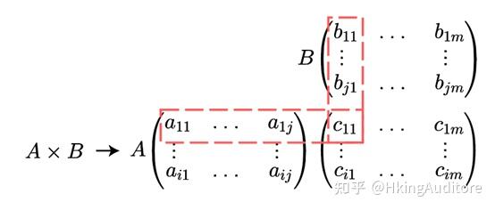
根据上文中我们给出了矩阵与向量相乘的算法,让我们总结出矩阵相乘的计算式吧:
其中,
c_{\text{μλ}} = a_{\text{μi}} \cdot b_{1\lambda} + a_{\mu 2} \cdot b_{2\lambda} + \cdots + a_{\mu j} \cdot b_{\text{jλ}}
矩阵乘法拥有以下性质:
\left( \mathbf{\text{AB}} \right)\mathbf{C}\mathbf{=}\mathbf{A}\left( \mathbf{\text{BC}} \right)
是一个有序的空间变换;因为矩阵乘法的目的是得到与两次矩阵变换等价的变换;所以不仅可以先求
向量组在
中的表示,再求得到的
向量组在
的表示;还可以先求
共同表示的空间,再求
向量组在空间
的表示。
\mathbf{\lambda}\left( \mathbf{\text{AB}} \right)\mathbf{=}\left( \mathbf{\text{λA}} \right)\mathbf{B}\mathbf{=}\mathbf{A}\left( \mathbf{\text{λB}} \right)
将标量相乘意味着只对变换进行缩放而不改变空间的网格结构。用列向量形式进行理解:在
\left( \text{λA} \right)B
中,先对
进行缩放,当
的列向量进行
变换时,缩放量
自然也会间接作用到列向量上;而对
A\left( \text{λB} \right)
,先对
中的列向量进行缩放,当变换
进行时,缩放量
自然也随着向量一起变换。
\mathbf{A}\left( \mathbf{B}\mathbf{+}\mathbf{C} \right)\mathbf{=}\mathbf{\text{AB}}\mathbf{+}\mathbf{\text{AC}}
意味着在初始坐标系下将
与
向量组相加,再在
空间中解释
与
向量组相加后的结果;而
意味着先在A空间中取
,
,再在初始坐标系将它们相加,还是以列向量视角看,在上一节讲述矩阵与向量乘时用了"参照"的概念,而矩阵是一种线性变化,并不改变两个向量间的“相对关系"(可以想象成变换后的新坐标轴仍有对应"平行关系")。因此分配律是成立的。
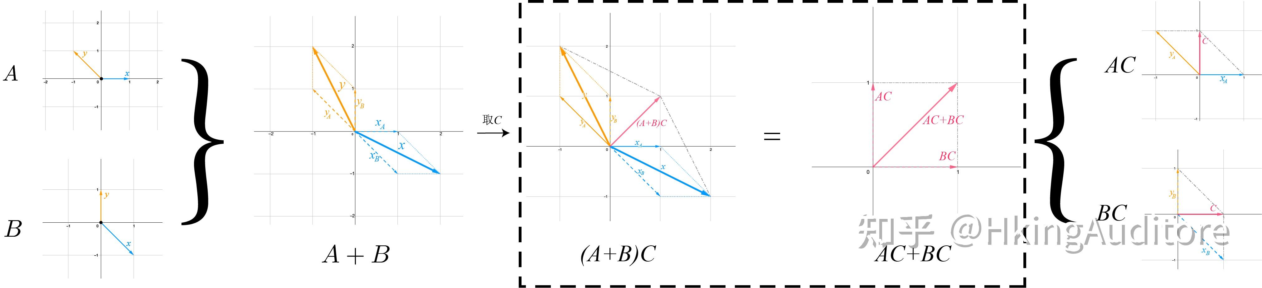
\left( \mathbf{A + B} \right)\mathbf{C = AC + BC}
意即在初始坐标系下将
与
相加,再于新空间中对
中的列向量进行解释。
意即分别在
与
变换后的空间中解释
中的列向量,再在初始坐标系下将向量组相加。由于
与
变换都基于在同一坐标系表述,因此它们描述的基向量变换可以合并使用也可拆分使用。
举个例子,假设有变换
、
,以及
:
另假设有向量
C\begin{pmatrix} 1 \\ 1 \\ \end{pmatrix}
,则
、
和
表现为:
现在,若我们试图在
中取
,则会发现它们其实是同样的向量:
\mathbf{\text{AB}} = \mathbf{0}
不意味着
或
?
意即经过
,
两次变换后,新空间中所有向量都指向了原点,即转至零维空间。根据之前所学,这个过程可以是逐次降维,比如,
先将
轴压至0,
再将
轴压至0;再比如,
变换是将三维向量降维到仅有
轴一维,
变换是将三维向量降维到仅有
平面,但由于变化进行到
时已无
平面,所以
变换就表现为把空间经由
变换后剩下的
轴降维到原点了。
所以,若存在
,我们可以肯定的是
过程一定降了维,但不一定是
或者
一次性把所有维数降为0,也不一定是
各自降维数之和就是目标空间的维数;只能说是
与
各自降维的并集大于目标空间的维数。
也就是说,当两个矩阵相乘为0,则两个矩阵的总降维数大于等于向量/空间的维度。
这个问题可看作是上一个问题的推广,翻译成符号形式就是如果
,为什么没有
?
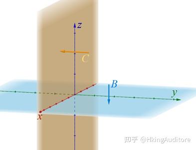
我们设
代表着一个三维空间的向量组,而
矩阵表示一个将三维空间
\begin{pmatrix} 1 & 0 & 0 \\ 0 & 1 & 0 \\ 0 & 0 & 1 \\ \end{pmatrix}
降维至二维空间
\begin{pmatrix} 1 & 0 \\ 0 & 1 \\ \end{pmatrix}
(
面)的变化,
矩阵表示一个将空间降维至
\begin{pmatrix} 1 & 0 \\ 0 & 0 \\ 0 & 1 \\ \end{pmatrix}
(
面)面的变化,即
矩阵让
轴归零,
矩阵让
轴归零。
也就是说,
面所有向量在
的作用下与
轴重合,
面所有向量都在
作用下与
轴重合。
现在,在经由
变换或
变换后的空间中假设有一个在
轴上的向量
\begin{pmatrix} 1 \\ 0 \\ 0 \\ \end{pmatrix}
,你知道它是由哪个向量经哪个过程得到的吗?可以是
\begin{pmatrix} 1 \\ 0 \\ 1 \\ \end{pmatrix}
经
变换得到,也可以是
\begin{pmatrix} 1 \\ 1 \\ 0 \\ \end{pmatrix}
经
变换得到,它们结果都是
\begin{pmatrix} 1 \\ 0 \\ \end{pmatrix}
,但我们根本无法不知道它是原来的位置。
在这里,我们找到了一个满足
的变换,他们的作用效果都是将三维空间降维到二维空间,而且我们也找了一个这两个空间共用的向量
\begin{pmatrix} 1 \\ 0 \\ 0 \\ \end{pmatrix}
,但显然
和
是两个完全不同的变换,即
。
也就是说,对于出现了降维变化的过程,由于存在多个源对应同一结果的情况,因此不能由同一结果就想当然地得出它们经历了同一变换。
矩阵的秩
我们在第一章中讲了向量组的秩概念,因此在矩阵中,我们也自然而然地联想到了它。
在矩阵中,对于一个矩阵
,存在一个能与
作用的最大维度空间
,
的维数就是矩阵的秩。
这个概念读起来很拗口,不过它和向量组的秩概念是类似的。如果我们将矩阵当作列向量组处理,那其对应列向量组的秩就是矩阵的秩,因为我们可以把矩阵各列看成"基向量变化后的位置",所以理解这个概念其实并不难。
下面看几个关于秩的有趣性质
\mathbf{0 \leq}\mathbf{R}\left( \mathbf{A}_{\mathbf{m}\mathbf{\times}\mathbf{n}} \right)\mathbf{\leq}\mathbf{\min}\left\{ \mathbf{m}\mathbf{,}\mathbf{n} \right\}
由向量组知识:
维向量最多张成
维空间,
个向量最多张成
维空间,两者相互制约,故取最小。
\mathbf{R}\left( \mathbf{A} \right)\mathbf{=}\mathbf{R}\left( \mathbf{\text{kA}} \right)\left( \mathbf{k}\mathbf{\neq 0} \right)
缩放不影响空间维度
中某行/列得到
,则
\mathbf{R}\left( \mathbf{B} \right) \leq \mathbf{R}\left( \mathbf{A} \right)
由①可证出
是
\mathbf{m} \times \mathbf{n}
阵,
,
分别是
阶,
阶不表示降维过程的矩阵,则
\mathbf{R}\left( \mathbf{A} \right) = \mathbf{R}\left( \mathbf{\text{PA}} \right) = \mathbf{R}\left( \mathbf{\text{AQ}} \right) = \mathbf{R}\left( \mathbf{\text{PAQ}} \right)
进行一个不降维的变换,结果的维数一定不变。
\mathbf{M}\mathbf{\text{ax}}\left\{ \mathbf{R}\left( \mathbf{A} \right),\mathbf{R}\left( \mathbf{B} \right) \right\} \leq \mathbf{R}\left( \mathbf{A},\mathbf{B} \right) \leq \mathbf{R}\left( \mathbf{A} \right) + \mathbf{R}\left( \mathbf{B} \right)
(1) 由向量组知识,合并两个向量组
,
得到新向量组,若
表示
的子空间,则
R\left( \text{AB} \right) = R(B)
,反之,若
R\left( \text{AB} \right) = R(B)
,则
表示
的子空间。若存在
个维度只能由
或
其一表示,则
或
的组合空间一定比原
或
空间多出这
个维度,即
R(A,B) > M\text{ax}\left\{ R(A),R(B) \right\}
,且有
R(A,B) = M\text{ax}\left\{ R(A),R(B) \right\} + n
。 综上
R(A,B) \geq M\text{ax}\left\{ R(A),R(B) \right\}
(2)若
与
有一秩为0,则
。若组合
与
两个向量组出现维度交集,即存在维度
,则计算
时,
会受到抵消,则显然
\mathbf{R}\left( \mathbf{A} + \mathbf{B} \right) \leq \mathbf{R}\left( \mathbf{A} \right) + \mathbf{R}\left( \mathbf{B} \right)
即对组成
,
各自的向量进行相加。
设
A\left( \alpha_{1},\alpha_{2}\cdots,\alpha_{n} \right)
,
B\left( \beta_{1},\beta_{2},\cdots,\beta_{n} \right)
则
A + B = (\alpha_{1} + \beta_{1},\alpha_{2} + \beta_{2},\ldots ,\alpha_{n} + \beta_{n})
,
(A,B) = \left( \alpha_{1},\alpha_{2}\cdots,\alpha_{n},\beta_{1},\beta_{2},\cdots\beta_{n} \right)
因为
中所有的向量都可以用
中的向量线性表示,所以
是
的子空间。也就是说,
。
又因为
,所以
R(A + B) \leq R(A) + R(B)
。
\mathbf{A}_{\mathbf{m} \times \mathbf{n}}\mathbf{B}_{\mathbf{n} \times \mathbf{c}} = \mathbf{0}
,则
\mathbf{R}\left( \mathbf{A} \right) + \mathbf{R}\left( \mathbf{B} \right) \leq \mathbf{n}
这个性质在矩阵乘法那一节中给过类似的证明,但新概念的引入可以给出更好的证明。
因为
,则
表示将一个名义
维向量组
转至0维。
设
变化使
维空间降低了
维,则
。
因为存在
(名义维数减去实际减少的维数即为真实维数),则
R(A) + R(B) = n - \lambda + R(B) \leq n - \lambda + \lambda = n
\mathbf{R}\left( \mathbf{\text{AB}} \right) \leq \mathbf{m}\mathbf{\text{in}}\left\{ \mathbf{R}\left( \mathbf{A} \right),\mathbf{R}\left( \mathbf{B} \right) \right\}
设
为
矩阵,
为
矩阵,则
为
矩阵,
矩阵将向量组
中的
个
维向量转为
个
维向量。
(1)若
矩阵表示升维过程
由向量组知识可知,
中只存在
个基,其余的
个向量均可由
个基表示。当
对
中的基进行变换时,其余的
个向量依旧在
个基张成空间的子空间内,故秩不变。
(2)若
矩阵表示降维过程
与1类似,
对
中
个基进行了降维,即
中
个基张成空间的名义维度降至
维,由此可知
R\left( \text{AB} \right)
不大于
。
设存在维度
,在原向量组
中,假设存在两个基向量
和基向量
,
和
满足在消除
分量后线性相关。若
在经由
变换后被归零,则
和
将线性相关,则
。
又因为
矩阵表示降维过程,则
,故此时满足
R\left( \text{AB} \right) \leq m\text{in}\left\{ R(A),R(B) \right\}
。
(3)若
矩阵不改变维数
根据上文,可知此时
R\left( \text{AB} \right) = R(B)
。
综上所述
\mathbf{R}\left( \mathbf{\text{AB}} \right)\mathbf{\leq}\mathbf{m}\mathbf{\text{in}}\left\{ \mathbf{R}\left( \mathbf{A} \right)\mathbf{,}\mathbf{R}\left( \mathbf{B} \right) \right\}