GEE非参数趋势分析（Mk-Sen）

Twcat_tree

发布于 2024-04-15 09:17:39

2280

发布于 2024-04-15 09:17:39

趋势分析是寻找感兴趣的东西正在增加的地方，或者减少多少。更具体地说，本教程演示了使用非参数 Mann-Kendall 检测影像中的单调趋势测试是否存在增加或减少的趋势以及 Sen 的斜率量化趋势的幅度（如果存在）。本教程还显示估计 Mann-Kendall 检验统计量的方差，Mann Kendall 检验统计量是检验是否存在任何趋势，以及统计量的 P 值（假设正态分布）。重要提示：此处介绍的方法适用于评估单调趋势（即没有季节性的数据）在离散数据中（即非浮点）。此外，如果应用本教程中的方法对新数据（即地区、时间范围、来源）可以需要调整和可视化参数以适应特别的结果。

时间序列数据 我们将使用来自MOD13A1数据集的MODIS增强植被指数（EVI）的时间序列。此图像集合的每个像素都包含一个时间序列，我们将计算每个像素的统计信息。假设将集合筛选为一个季节足以获得具有单调趋势的时间序列。自检查该假设是否适用于您感兴趣的领域，添加收集到地图并使用检查器，单击一些点并查看控制台中显示的系列图表。根据需要调整过滤器。

var mod13 = ee.ImageCollection('MODIS/006/MOD13A1');
var coll = mod13.select('EVI')
    .filter(ee.Filter.calendarRange(8, 9, 'month'));
Map.setCenter(-121.6, 37.3, 10);
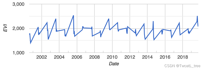
Map.addLayer(coll, {min: -500, max: 5000, palette: ['white', 'green']}, 'coll');

此集合中的 EVI 时间序列（一个像素）示例如下所示。是这个像素有趋势吗？更重要的是，从统计学上讲，这是一个这个像素的显着趋势？请继续阅读，找出答案！

EVI time series in a single pixel

将时间序列连接到自身 感兴趣的非参数统计是通过检查所有可能的来计算的时间序列中唯一值的排序对。如果有 n 个时间点在序列中，我们需要检查 N（N-1）/2 对（i， j），i<j，其中 i 和 j 是任意时间索引。（这里我们用（i，j）来表示由 i 和 j 索引的一对 EVI 图像）。为此，请将集合加入到本身带有时间过滤器。时态过滤器将通过所有按时间顺序排列的后期图像。在联接的集合中，每个图像都将将它之后的所有图像存储在属性中。after

var afterFilter = ee.Filter.lessThan({
  leftField: 'system:time_start',
  rightField: 'system:time_start'
});

var joined = ee.ImageCollection(ee.Join.saveAll('after').apply({
  primary: coll,
  secondary: coll,
  condition: afterFilter
}));

Mann-Kendall 趋势检验 Mann-Kendall 趋势定义为所有货币对的符号之和。如果时间 j 的 EVI 大于时间 i 的 EVI，则为 1，如果相反是真的，否则为零（如果它们相等）。计算方式循环访问集合并计算集合中的每个图像和图像中的每个图像。signsign(i, j)ijafter

var sign = function(i, j) { // i and j are images
  return ee.Image(j).neq(i) // Zero case
      .multiply(ee.Image(j).subtract(i).clamp(-1, 1)).int();
};

var kendall = ee.ImageCollection(joined.map(function(current) {
  var afterCollection = ee.ImageCollection.fromImages(current.get('after'));
  return afterCollection.map(function(image) {
    // The unmask is to prevent accumulation of masked pixels that
    // result from the undefined case of when either current or image
    // is masked.  It won't affect the sum, since it's unmasked to zero.
    return ee.Image(sign(current, image)).unmask(0);
  });
  // Set parallelScale to avoid User memory limit exceeded.
}).flatten()).reduce('sum', 2);

var palette = ['red', 'white', 'green'];
// Set min and max stretch visualization parameters as necessary.
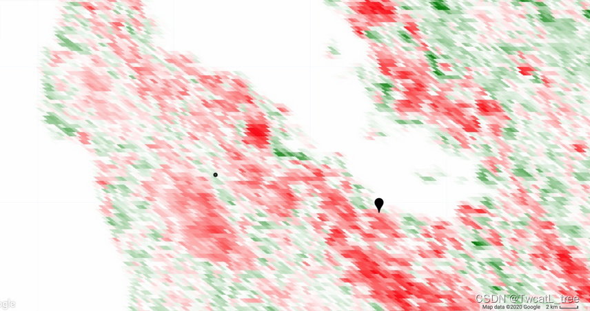
Map.addLayer(kendall, {palette: palette, min: -2800, max: 2800}, 'kendall');

缩放到您感兴趣的区域并定义大致对称的颜色拉伸使用地图图层样式设置对话框（即和的均值近似为零）。红色像素呈递减趋势，绿色像素呈递减趋势像素呈增加趋势。如下图所示美国加利福尼亚州一个地区的 Mann-Kendall 统计量。地图图钉是在 Googleplex 的大致位置。该点是从中提取上述时间序列的点。我们想要以确定此地图中的哪些像素具有显著趋势。minmax

您可能还想知道趋势的幅度或斜率在当前背景下随时间推移的趋势。一种非参数化方式用森的斜率来评估。

森氏斜坡 Sen 斜率的计算方式与 Mann-Kendall 统计量类似。但是，不是将所有符号对相加，而是计算斜率对于所有对。Sen 斜率是所有这些对的中位斜率。在在下文中，斜率是以天为单位计算的，以避免数值上的微小斜率（这可能是由于改用纪元时间而产生的）。

var slope = function(i, j) { // i and j are images
  return ee.Image(j).subtract(i)
      .divide(ee.Image(j).date().difference(ee.Image(i).date(), 'days'))
      .rename('slope')
      .float();
};

var slopes = ee.ImageCollection(joined.map(function(current) {
  var afterCollection = ee.ImageCollection.fromImages(current.get('after'));
  return afterCollection.map(function(image) {
      return ee.Image(slope(current, image));
  });
}).flatten());

var sensSlope = slopes.reduce(ee.Reducer.median(), 2); // Set parallelScale.
Map.addLayer(sensSlope, {palette: palette, min: -1, max: 1}, 'sensSlope');

要获取 Sen 的截距（如果需要），请计算所有截距并取中位数。

var epochDate = ee.Date('1970-01-01');
var sensIntercept = coll.map(function(image) {
  var epochDays = image.date().difference(epochDate, 'days').float();
  return image.subtract(sensSlope.multiply(epochDays)).float();
}).reduce(ee.Reducer.median(), 2);
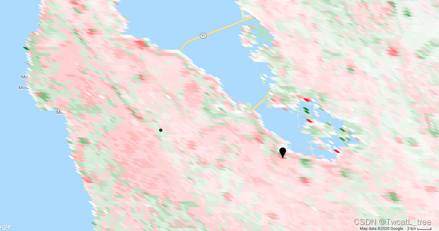
Map.addLayer(sensIntercept, {min: -6600, max: 20600}, 'sensIntercept');

森的斜坡图如下所示。请注意，该模式类似于 Mann-Kendall 统计量，但不完全相同。此外，还有哪些像素具有显着趋势的问题，这个问题将很快得到答复。

前面的示例仅用于演示计算。如果你需要 Sen 的斜率和/或截距，您还可以使用 Sen 的斜率减速器，它可能更容易（更少的代码）和更高的效率，但计算 intercept 作为通过中位数的线的 y 值。

Mann-Kendall 统计量的方差 计算 Mann-Kendall 统计量的方差时，由于数据中可能存在联系（即等于零）。计算这些关系可能会有点棘手，需要基于数组前向差分。请注意，您可以在计算中评论您是否不关心领带和想要忽略该更正。sign(i, j).subtract(groupFactorSum)kendallVariance

// Values that are in a group (ties).  Set all else to zero.
var groups = coll.map(function(i) {
  var matches = coll.map(function(j) {
    return i.eq(j); // i and j are images.
  }).sum();
  return i.multiply(matches.gt(1));
});

// Compute tie group sizes in a sequence.  The first group is discarded.
var group = function(array) {
  var length = array.arrayLength(0);
  // Array of indices.  These are 1-indexed.
  var indices = ee.Image([1])
      .arrayRepeat(0, length)
      .arrayAccum(0, ee.Reducer.sum())
      .toArray(1);
  var sorted = array.arraySort();
  var left = sorted.arraySlice(0, 1);
  var right = sorted.arraySlice(0, 0, -1);
  // Indices of the end of runs.
  var mask = left.neq(right)
  // Always keep the last index, the end of the sequence.
      .arrayCat(ee.Image(ee.Array([[1]])), 0);
  var runIndices = indices.arrayMask(mask);
  // Subtract the indices to get run lengths.
  var groupSizes = runIndices.arraySlice(0, 1)
      .subtract(runIndices.arraySlice(0, 0, -1));
  return groupSizes;
};

// See equation 2.6 in Sen (1968).
var factors = function(image) {
  return image.expression('b() * (b() - 1) * (b() * 2 + 5)');
};

var groupSizes = group(groups.toArray());
var groupFactors = factors(groupSizes);
var groupFactorSum = groupFactors.arrayReduce('sum', [0])
      .arrayGet([0, 0]);

var count = joined.count();

var kendallVariance = factors(count)
    .subtract(groupFactorSum)
    .divide(18)
    .float();
Map.addLayer(kendallVariance, {min: 1700, max: 85000}, 'kendallVariance');

显著性检验 Mann-Kendall 统计量对于适当大样品。假设我们的样本足够大且不相关。在这些之下假设，Mann-Kendall 统计量的真实均值为零，并且方差如上计算。要计算标准正态统计量（），将统计量除以其标准差。z 统计量的 P 值（观察到这种极值的概率）是 1 - P（|z| < Z）。为对是否存在任何趋势（正或负）的双侧测试 95% 置信水平，将 P 值与 0.975 进行比较。（或者，比较 Z* 的 z 统计量，其中 Z* 是逆分布函数 0.975）。z

标准正态分布函数可以在 Earth Engine 中计算得出 error 函数 .分布函数及其逆函数如下所示以供参考。在这里，我们使用分布函数得到 1 - P（|z| < Z）并将其与 0.975 进行比较。erf()

// Compute Z-statistics.
var zero = kendall.multiply(kendall.eq(0));
var pos = kendall.multiply(kendall.gt(0)).subtract(1);
var neg = kendall.multiply(kendall.lt(0)).add(1);

var z = zero
    .add(pos.divide(kendallVariance.sqrt()))
    .add(neg.divide(kendallVariance.sqrt()));
Map.addLayer(z, {min: -2, max: 2}, 'z');

// https://en.wikipedia.org/wiki/Error_function#Cumulative_distribution_function
function eeCdf(z) {
  return ee.Image(0.5)
      .multiply(ee.Image(1).add(ee.Image(z).divide(ee.Image(2).sqrt()).erf()));
}

function invCdf(p) {
  return ee.Image(2).sqrt()
      .multiply(ee.Image(p).multiply(2).subtract(1).erfInv());
}

// Compute P-values.
var p = ee.Image(1).subtract(eeCdf(z.abs()));
Map.addLayer(p, {min: 0, max: 1}, 'p');

// Pixels that can have the null hypothesis (there is no trend) rejected.
// Specifically, if the true trend is zero, there would be less than 5%
// chance of randomly obtaining the observed result (that there is a trend).
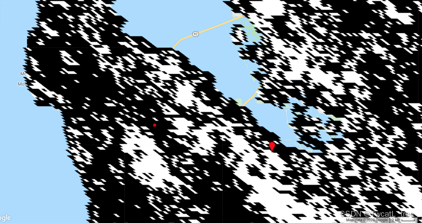
Map.addLayer(p.lte(0.025), {min: 0, max: 1}, 'significant trends');

下面显示了“有效”像素（白色）的映射，或通过测试的像素。如果我们的假设是正确的并且您对计算感到满意，您可能希望处理这些像素不同，用作蒙版。请注意，像素上面显示的时间序列（下图中的红色）没有显著趋势。p.lte(0.025)p.lte(0.025)