从零开始的异世界生信学习 R语言部分 05 作图-1
原创
从零开始的异世界生信学习 R语言部分 05 作图-1
原创
用户10361520
发布于 2023-03-05 22:21:22
发布于 2023-03-05 22:21:22
1.常用的可视化R包
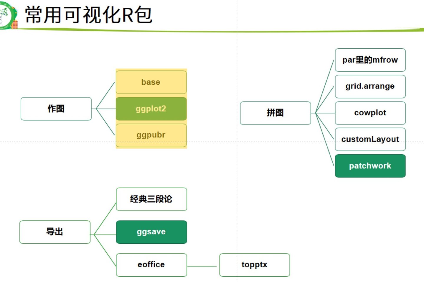
可视化R包
2.三种R包的作图函数
#作图分三类

#1.基础包 略显陈旧 了解一下
plot(iris[,1],iris[,3],col = iris[,5])
text(6.5,4, labels = 'hello')

dev.off() #关闭画板

#2.ggplot2 中坚力量,语法有个性
library(ggplot2)
ggplot(data = iris)+
  geom_point(mapping = aes(x = Sepal.Length,
                           y = Petal.Length,
                           color = Species))

#3.ggpubr 新手友好型 ggplot2简化和美化 褒贬不一
library(ggpubr)
ggscatter(iris,
          x="Sepal.Length",
          y="Petal.Length",
          color="Species")
3.ggplot2语法
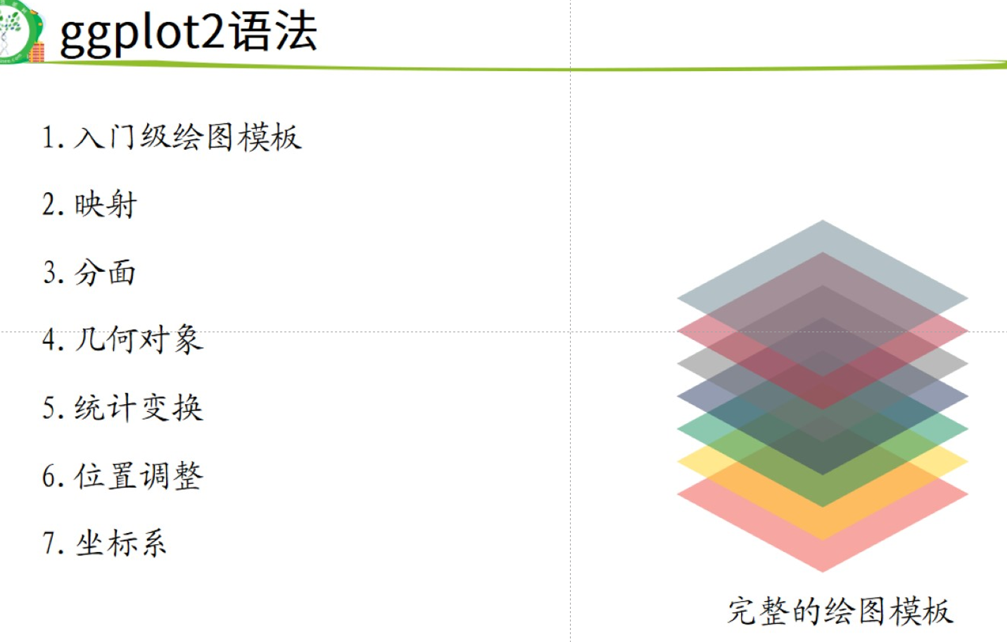
3.1入门级基础语法规则
ggplot2 入门级语法
ggplot2的特殊语法规则:列名不带引号,行末写加号(加号表示不同函数之间的连接)
library(ggplot2)
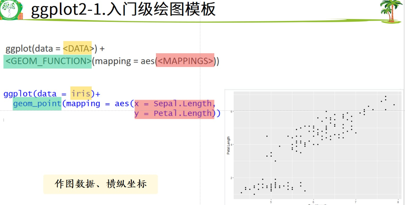
#1.入门级绘图模板:作图数据,横纵坐标
ggplot(data = iris)+
geom_point(mapping = aes(x = Sepal.Length,
y = Petal.Length))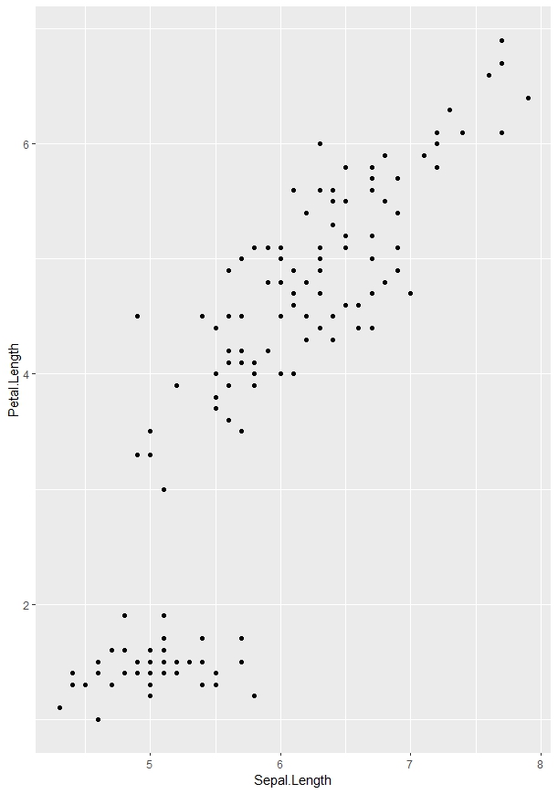
3.2属性设置(颜色、大小、透明度、点的形状,线型等)
3.2.1手动设置,需要设置为有意义的值
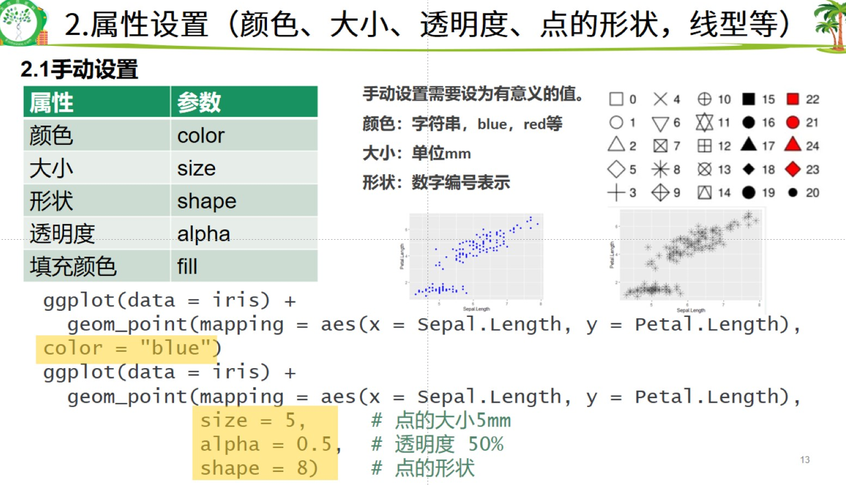
属性设置
color 颜色,可以用RGB编码值的字符串
size 大小,只能用数字
shape 形状,数字编号
alpha 透明度,0<x<1的数字
fill 填充颜色
只能全部统一设置
ggplot(data = iris) +
  geom_point(mapping = aes(x = Sepal.Length,
                           y = Petal.Length),
             color = "blue")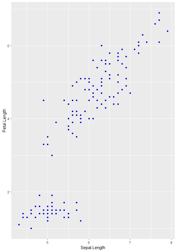
ggplot(data = iris) +
  geom_point(mapping = aes(x = Sepal.Length, y = Petal.Length),
             size = 5,     # 点的大小5mm
             alpha = 0.5,  # 透明度 50%
             shape = 8)  # 点的形状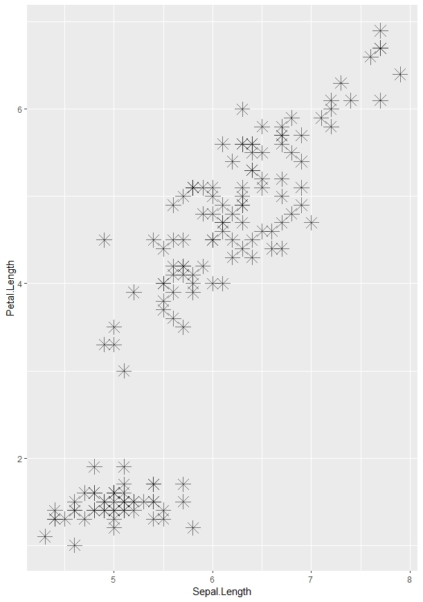
3.2.2 映射:按照数据框的某一列来定义图的某个属性
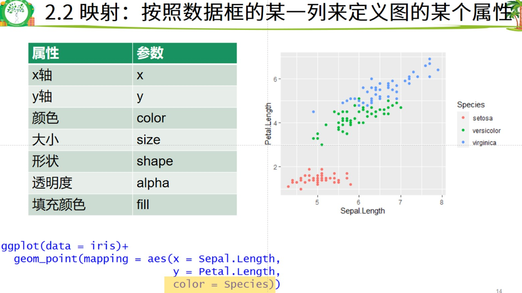
#2.2 映射:按照数据框的某一列来定义图的某个属性
ggplot(data = iris)+
  geom_point(mapping = aes(x = Sepal.Length,
                           y = Petal.Length,
                           color = Species))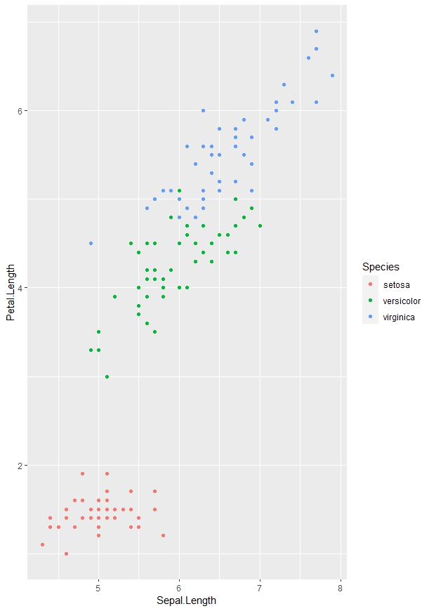
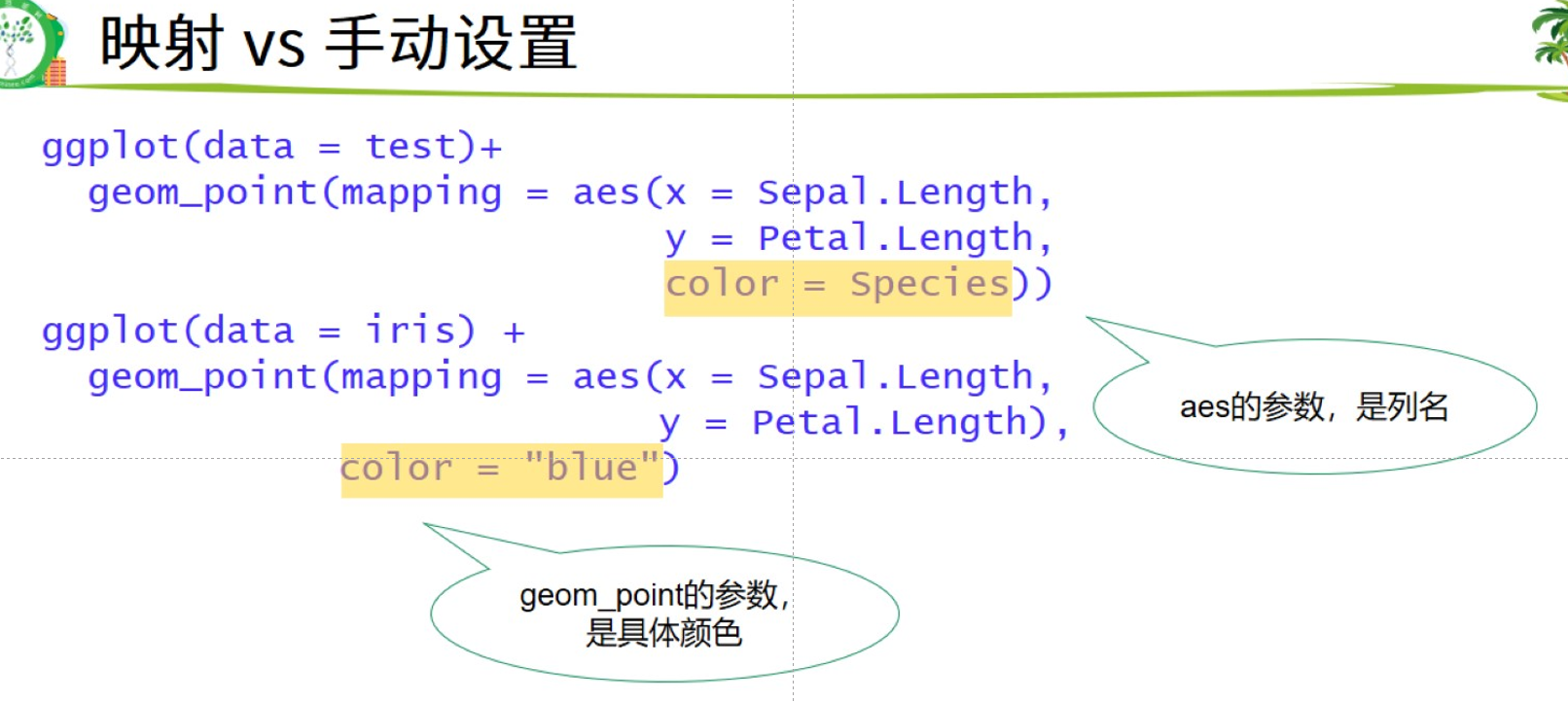
映射和手动输入的区别

映射和手动输入的区别
## Q1 能不能自行指定映射的具体颜色?

ggplot(data = iris)+
  geom_point(mapping = aes(x = Sepal.Length,
                           y = Petal.Length,
                           color = Species))+
  scale_color_manual(values = c("blue","grey","red"))
#color中的映射有多少个取值,manual应该就有几个颜色取值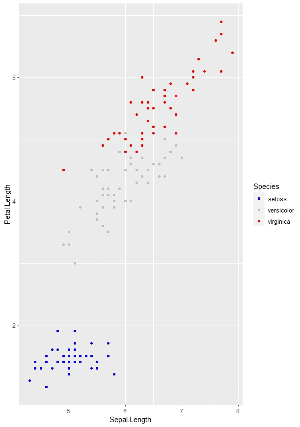
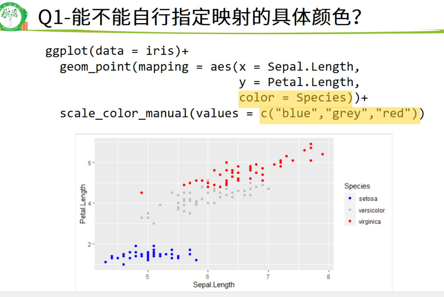
映射的取值
## Q2 区分color和fill两个属性
##color是颜色,fill是填充颜色
### Q2-1 空心形状和实心形状都用color设置颜色(形状中1-20都不需要填充颜色)
ggplot(data = iris)+
  geom_point(mapping = aes(x = Sepal.Length,
                           y = Petal.Length,
                           color = Species),
             shape = 17) #17号,实心的例子

ggplot(data = iris)+
  geom_point(mapping = aes(x = Sepal.Length,
                           y = Petal.Length,
                           color = Species),
             shape = 2) #2号,空心的例子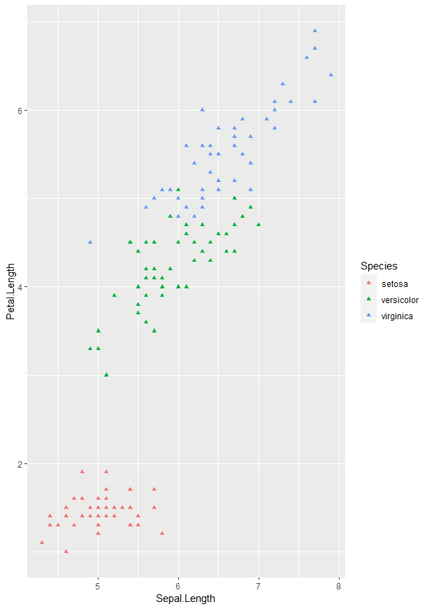
17号形状,实心

2号形状,空心
### Q2-2 既有边框又有内心的,才需要color和fill两个参数

ggplot(data = iris)+
  geom_point(mapping = aes(x = Sepal.Length,
                           y = Petal.Length,
                           color = Species),
             shape = 24,
             fill = "black") #24号,双色的例子,填充颜色为黑色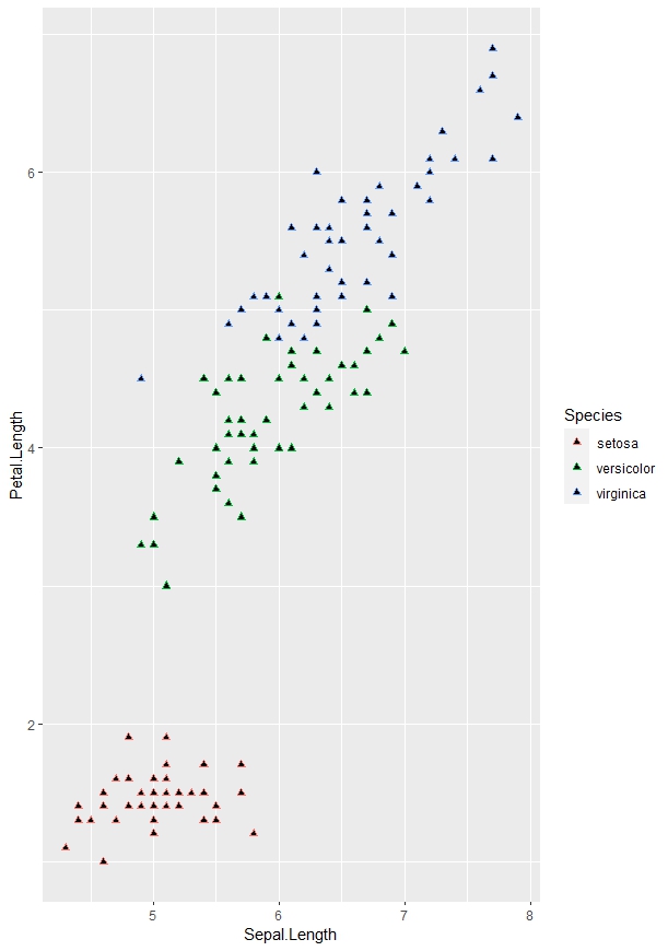
ggplot(data = iris)+
  geom_boxplot(mapping = aes(x = Species,
                           y = Sepal.Width,
                           fill= Species))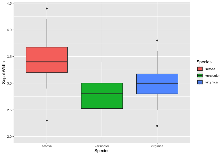
箱线图的颜色用fill函数填充
3.2.3 分面
#3.分面
ggplot(data = iris) +
  geom_point(mapping = aes(x = Sepal.Length, y = Petal.Length)) +
  facet_wrap(~ Species)
##分面是根据数据的某一列把一张图分成若干的子图,根据列的取值分成若干的图
##用来分面的列:1.应该是分类变量,离散型数据;2.取值数量有限;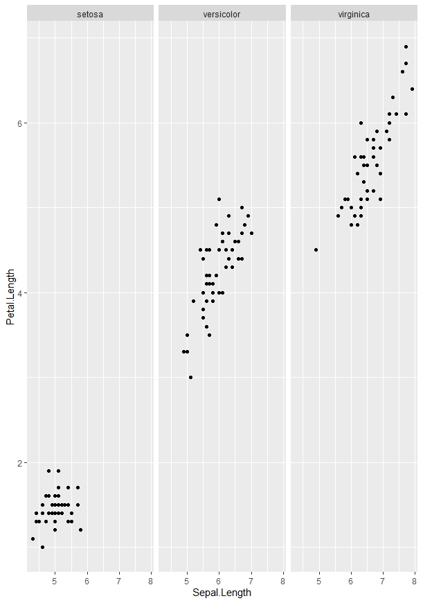
分面的图
#双分面
dat = iris
dat$Group = sample(letters[1:5],150,replace = T)
ggplot(data = dat) +
  geom_point(mapping = aes(x = Sepal.Length, y = Petal.Length)) +
  facet_grid(Group ~ Species)  #按照group列分隔行,species分隔列
  ##sample()函数表示随机取样
  ##dat$Group = sample(letters[1:5],150,replace = T) 表示在数据中新增了一列,其中按照内置数据letters(26个小写字母)中1-5(A-E)中可重复的取150个值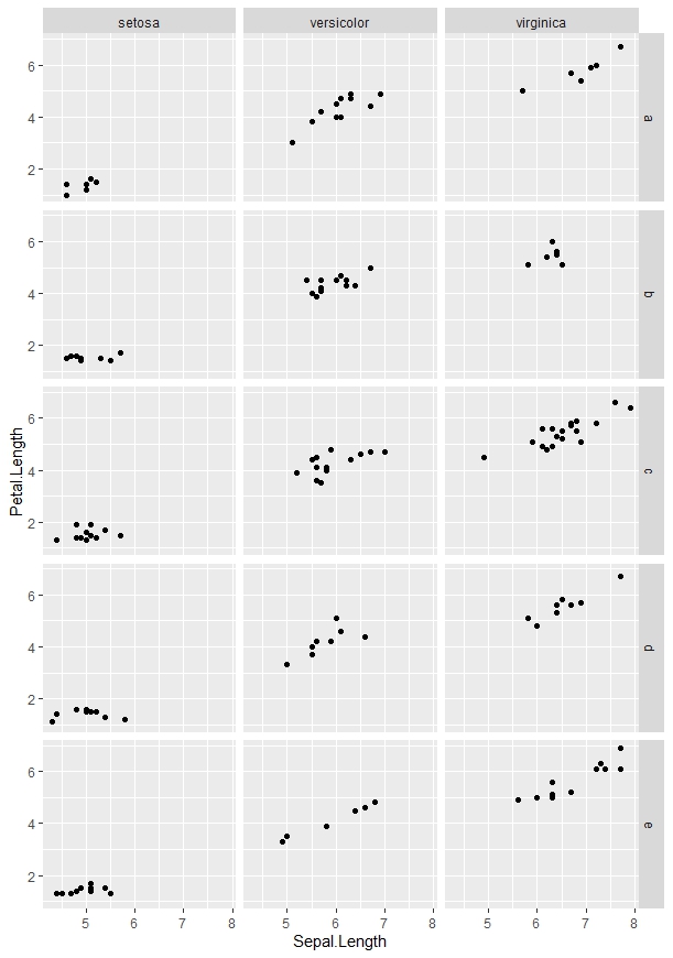
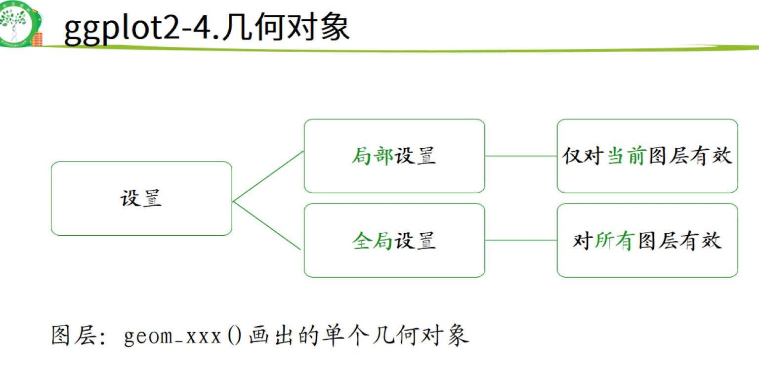
3.2.4 几何对象
指一个以geom开头的函数画出来的所有东西称为一个几何对象,也称为了一个图层
几何对象可以叠加
#4.几何对象

#局部设置和全局设置

ggplot(data = iris) +
  geom_smooth(mapping = aes(x = Sepal.Length,
                          y = Petal.Length))+
  geom_point(mapping = aes(x = Sepal.Length,
                           y = Petal.Length))  ##局部设置

ggplot(data = iris,mapping = aes(x = Sepal.Length, y = Petal.Length))+
  geom_smooth()+
  geom_point()  ##全局设置
##两种代码的图一样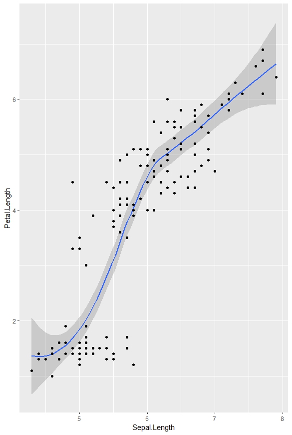
局部设置和全局设置
3.2.5 统计变换
#5.统计变换-直方图
View(diamonds)
table(diamonds$cut) ##内置数据钻石的切割质量

ggplot(data = diamonds) +
  geom_bar(mapping = aes(x = cut))  ##geom_bar函数默认没有y参数

ggplot(data = diamonds) +
  stat_count(mapping = aes(x = cut))
## 图片的横坐标为钻石切割质量,纵坐标为每个取值的格式。作图只需要一列
## geom开头的几何对象函数,stat开头的几何变换函数,两种函数存在对应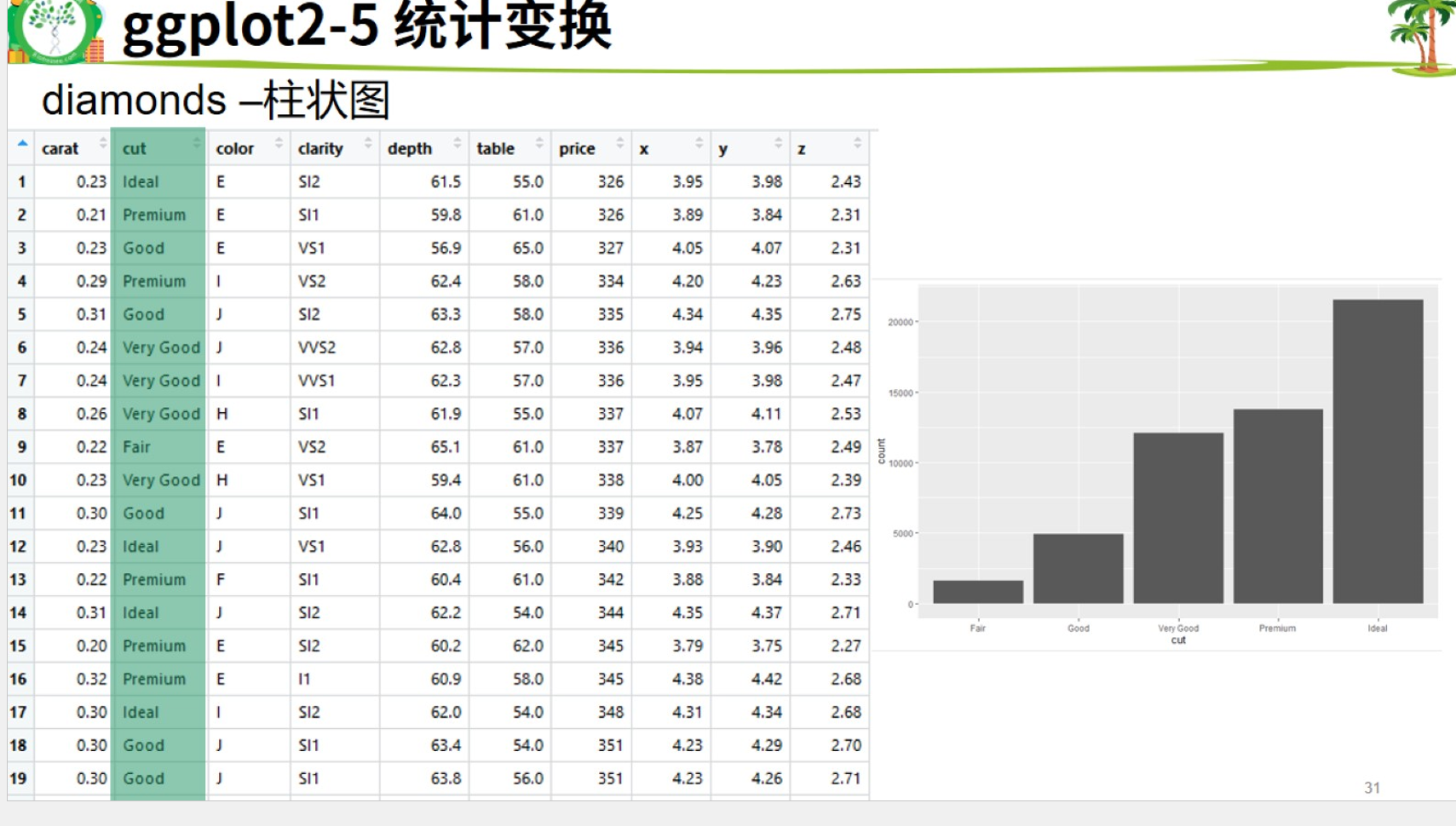
#统计变换使用场景
#5.1.不统计,数据直接做图
fre = as.data.frame(table(diamonds$cut))
fre

ggplot(data = fre) +
  geom_bar(mapping = aes(x = Var1, y = Freq), stat = "identity")
#5.2count改为prop,统计比例而不是具体数目,group参数表示分类统一比例
ggplot(data = diamonds) +
  geom_bar(mapping = aes(x = cut, y = ..prop.., group = 1))
3.2.6 位置关系
# 6.1抖动的点图
ggplot(data = iris,mapping = aes(x = Species,
                                 y = Sepal.Width,
                                 fill = Species)) +
  geom_boxplot()+
  geom_point()

ggplot(data = iris,mapping = aes(x = Species,
                                 y = Sepal.Width,
                                 fill = Species)) +
  geom_boxplot()+
  geom_jitter()   ##jitter绘制抖动的点图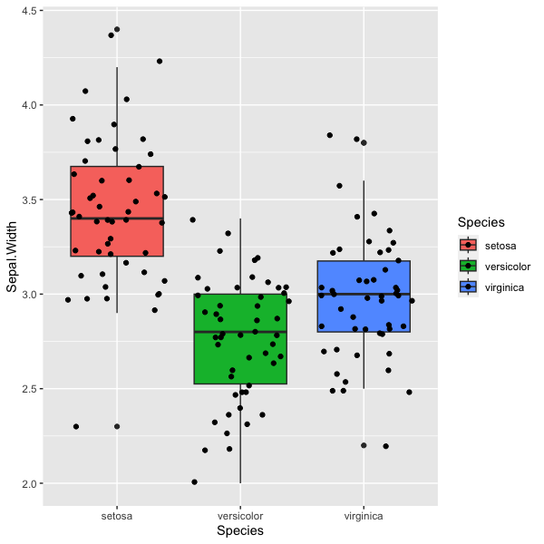
# 6.2堆叠直方图
ggplot(data = diamonds) +
  geom_bar(mapping = aes(x = cut,fill=clarity))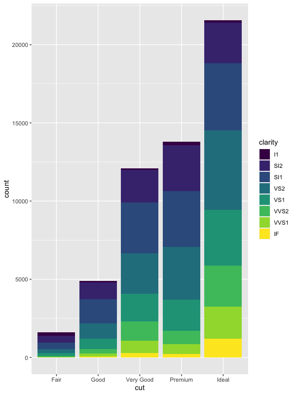
# 6.3 并列直方图
ggplot(data = diamonds) +
  geom_bar(mapping = aes(x = cut, fill = clarity), position = "dodge")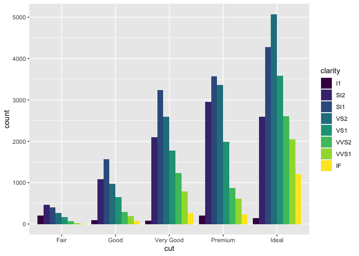
3.2.7 坐标系
#翻转coord_flip()

ggplot(data = mpg, mapping = aes(x = class, y = hwy)) +
  geom_boxplot() +
  coord_flip()
##可以实现X轴,Y轴的转换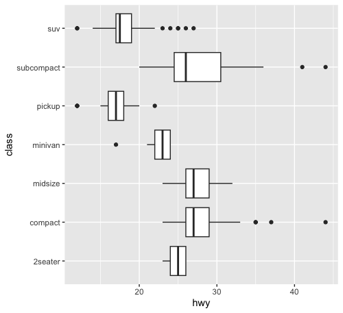
#极坐标系coord_polar()
bar <- ggplot(data = diamonds) +
  geom_bar(
    mapping = aes(x = cut, fill = cut),
    width = 1
  ) +
  theme(aspect.ratio = 1) +
  labs(x = NULL, y = NULL)
bar
bar + coord_flip()
bar + coord_polar()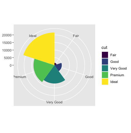
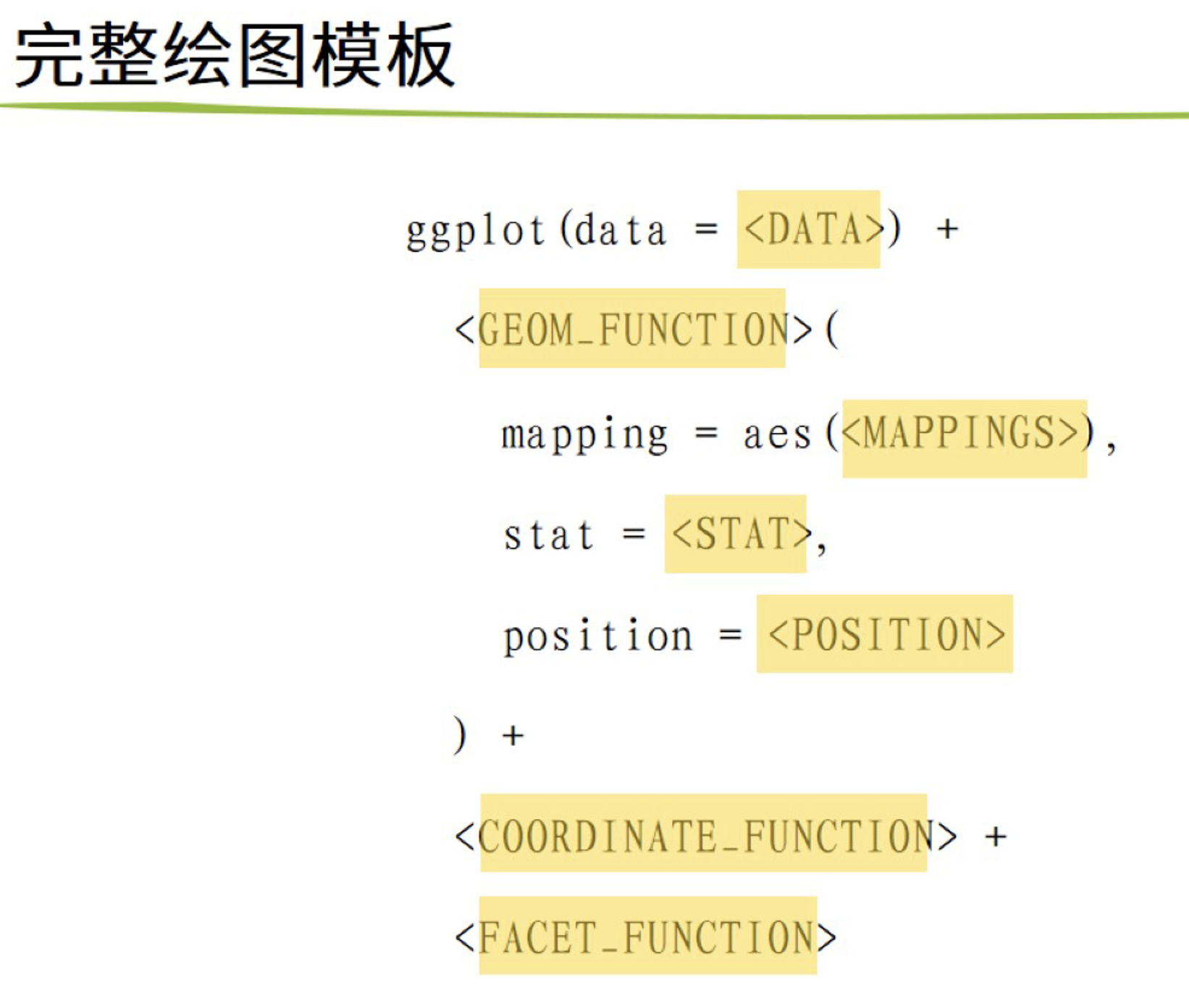
ggplot2 画图模板
##作图函数后面 +theme_classic() 可以去掉灰色的背景板
4. ggpubr 包
# ggpubr 搜代码直接用,基本不需要系统学习

# sthda上有大量ggpubr出的图
library(ggpubr)
ggscatter(iris,x="Sepal.Length",
          y="Petal.Length",
color="Species")p <- ggboxplot(iris, x = "Species",
y = "Sepal.Length",
color = "Species",
shape = "Species",
add = "jitter")
p ##ggplot2以及ggpubr绘制的图片可以进行赋值
my_comparisons <- list( c("setosa", "versicolor"),
c("setosa", "virginica"),
c("versicolor", "virginica") )
p + stat_compare_means(comparisons = my_comparisons)+ # Add pairwise comparisons p-value
stat_compare_means(label.y = 9) 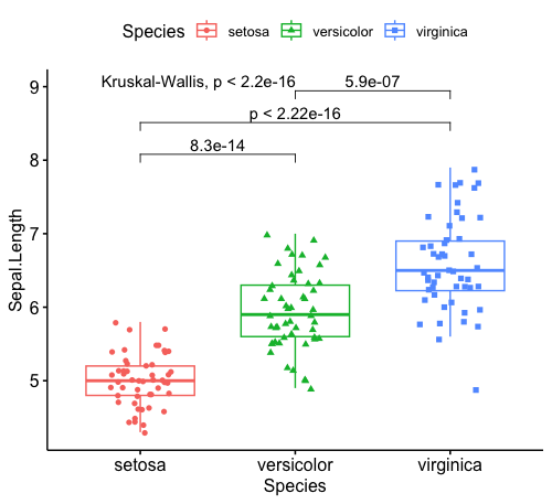
ggpubr 可以给箱线图添加组间比较的P值
ggplot(data = iris, mapping = aes(x = Species,
                                               y = Sepal.Width))+
  geom_violin(mapping = aes(fill = Species))+
  geom_boxplot()+
  geom_jitter(mapping = aes(shape = Species))+
  coord_flip()
#  也可以通过增加这个函数调整点图的点的形状 scale_shape_manual(values = c())
# 图层的叠放顺序取决于代码的顺序,先写的代码图片在最底下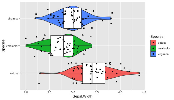
4.图片的保存和导出
#图片保存的三种方法

#1.基础包作图的保存
pdf("iris_box_ggpubr.pdf")
boxplot(iris[,1]~iris[,5])
text(6.5,4, labels = 'hello')
dev.off()

#2.ggplot系列图(包括ggpubr)通用的简便保存 ggsave
p <- ggboxplot(iris, x = "Species",
               y = "Sepal.Length",
               color = "Species",
               shape = "Species",
               add = "jitter")
ggsave(p,filename = "iris_box_ggpubr.png")
##保存的时候可以调节图片的参数,包括长宽以及像素,格式

#3.eoffice包 导出为ppt,全部元素都是可编辑模式
library(eoffice)
topptx(p,"iris_box_ggpubr.pptx")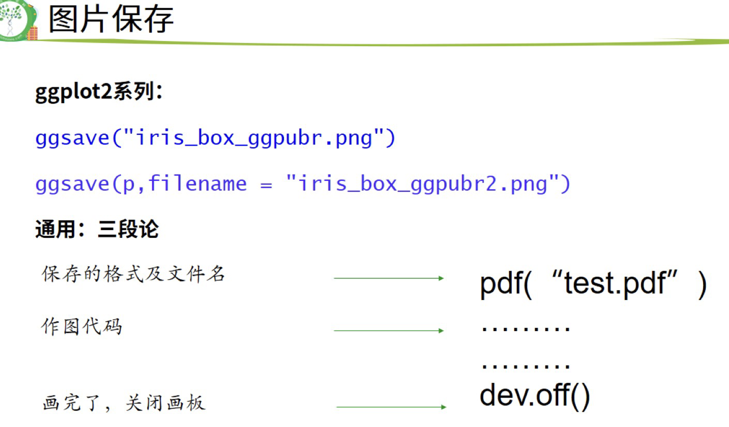
5.拼图
注意学习!!!

STHDA网站有很多作图代码
原创声明:本文系作者授权腾讯云开发者社区发表,未经许可,不得转载。
如有侵权,请联系 cloudcommunity@tencent.com 删除。
原创声明:本文系作者授权腾讯云开发者社区发表,未经许可,不得转载。
如有侵权,请联系 cloudcommunity@tencent.com 删除。
评论
登录后参与评论
推荐阅读
目录
腾讯云开发者
