R语言笔记-5

原创

Jon_L

修改于 2023-11-21 16:10:13

5450

修改于 2023-11-21 16:10:13

文章被收录于专栏：生信矿工

生信技能树-数据挖掘课程笔记

作图软件 base ggplot2 pheatmap ggvenn
拼图软件 patchwork
图片导出 经典三段函数 ggsave eoffice topptx

base 作图

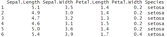
head(iris)
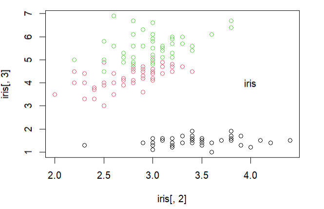
plot(iris[,2],iris[,3],col = iris[,5]) # 以内部数据iris的第2、3列分别作为横纵坐标绘制点图
text(4,4, labels = 'iris') #按坐标位置进行标记

输出结果：

base 作图函数

作图模板 plot() 散点图、折线图 hist() 频率直方图 boxplot() 箱线图 barplot() 柱状图 dotplot() 点图
映射

lines() 添加线

curve() 添加曲线

points() 添加点

axis() 坐标轴

title() 添加标题

text() 添加文字

ggplot2 作图

ggplot2是与base r语言不同的作图语法，最少元素包括：指定数据、美学映射、几何对象

ggplot2 基本元素

数据：作图的原始数据 ggplot(data = <DATA>)
几何对象：数据作图的图形方式 geom_<XXX>()
美学映射：图形的位置、颜色、大小、形状等 aes()
刻度：数据与美学映射的关系 scale()
统计转换：数据的统计作图 stat()
坐标系统：数据的坐标转换 coord()
面：数据的作图排列 facet_<XXX>()
主题：图形的背景、网格、轴、默认字体、大小等 theme()

library(ggplot2)
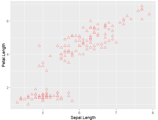
#以内部数据iris作图，Sepal.Length和Petal.Length分别作为横纵坐标
ggplot(data = iris) + 
    geom_point(mapping = aes(x = Sepal.Length,
                             y = Petal.Length), 
                color = "red", #点的颜色
                size = 2, #点的大小
                alpha = 0.5, #透明度
                shape = 24) #形状

输出结果：

ase() 常用属性：

属性	参数
颜色	color
大小	size
形状	shape
透明度	alpha
填充颜色	fill

点的形状与编号：

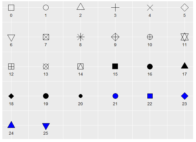
21-25分为边框与填充的颜色，参数color仅能控制边框的颜色，需设置参数fill的颜色

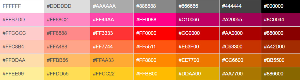
color() 可使用十六进制颜色代码

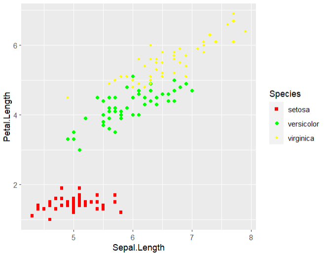
# 刻度函数可指定各自的颜色、大小等参数
ggplot(data = iris)+
    geom_point(mapping = aes(x = Sepal.Length,
                            y = Petal.Length,
                            color = Species,
                            shape= Species))+ # 映射：可按数据的某一列分组进行定义
    scale_color_manual(values = c("red","green","yellow"))+
    scale_shape_manual(values = c(15,16,18))

输出结果：

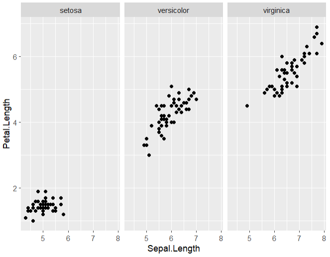
# 根据映射进行分面
ggplot(data = iris) + 
    geom_point(mapping = aes(x = Sepal.Length, y = Petal.Length)) + 
    facet_wrap(~ Species)

输出结果：

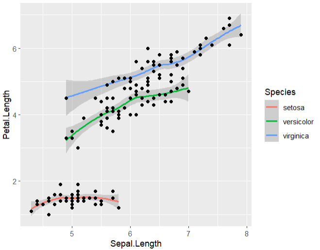
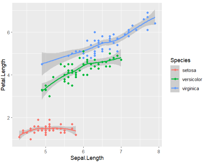
#局部设置
ggplot(data = iris)+
    geom_smooth(mapping = aes(x = Sepal.Length, 
                              y = Petal.Length,
                              color = Species))+
    geom_point(mapping = aes(x = Sepal.Length,
                             y = Petal.Length))
#全局设置
ggplot(data = iris,mapping = aes(x = Sepal.Length,
                                 y = Petal.Length,
                                 color = Species))+
    geom_smooth()+
    geom_point()

输出结果：

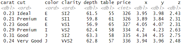
head(diamonds)
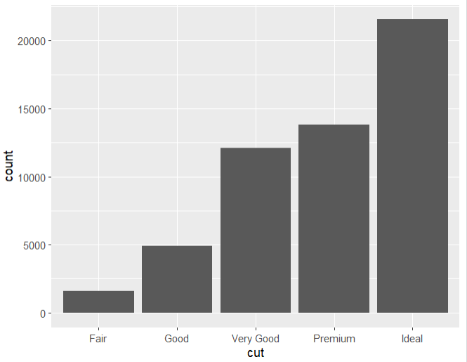
#两种函数均可统计内置数据diamonds中cut列的重复次数
ggplot(data = diamonds) + 
    geom_bar(mapping = aes(x = cut))

ggplot(data = diamonds) + 
    stat_count(mapping = aes(x = cut))

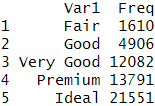
fre = table(diamonds$cut)
fre
#ggplot(data = fre) +
#  geom_bar(mapping = aes(x = Var1, y = Freq), stat = "identity") 
#  geom_bar()自动统计重复次数，若指定数值，需加入stat = "identity"

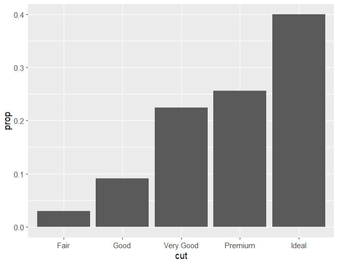
ggplot(data = diamonds) + 
    geom_bar(mapping = aes(x = cut, y = ..prop.., group = 1))#group = 1必选

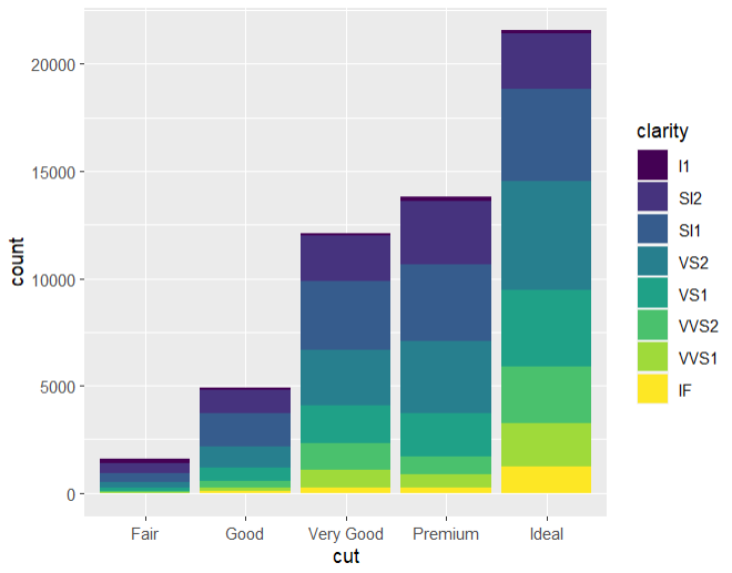
# 直方图指定映射，按比例堆叠
ggplot(data = diamonds) + 
    geom_bar(mapping = aes(x = cut,fill=clarity))

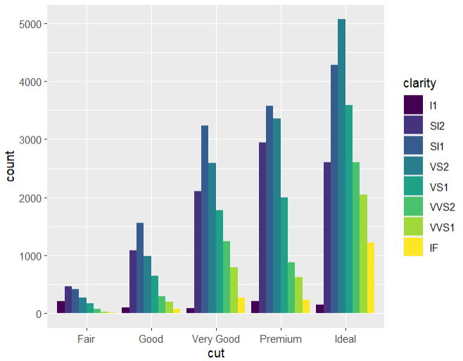
# 指定映射，直方图并列显示
ggplot(data = diamonds) + 
    geom_bar(mapping = aes(x = cut, fill = clarity), position = "dodge")

输出结果：

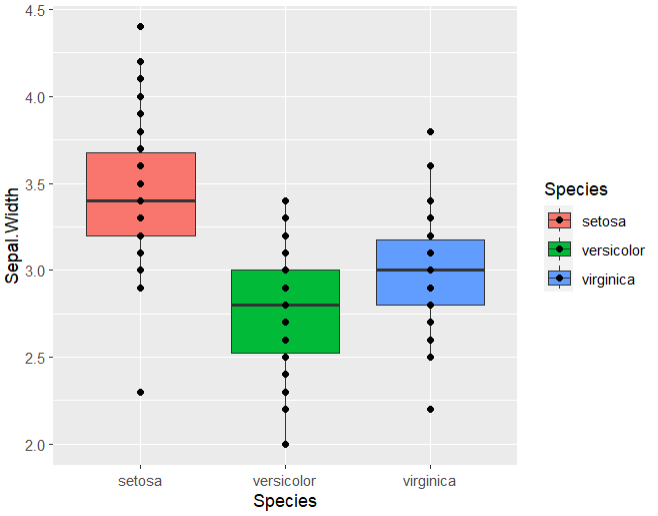
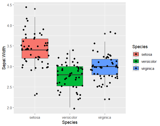
#绘制箱线图+点图（点集中于中线）
ggplot(data = iris,mapping = aes(x = Species, 
                                 y = Sepal.Width,
                                 fill = Species)) + 
    geom_boxplot()+
    geom_point()
#绘制箱线图+点图（点分散于中线周围，与中线的距离与数值无关）
ggplot(data = iris,mapping = aes(x = Species, 
                                 y = Sepal.Width,
                                 fill = Species)) + 
    geom_boxplot()+
    geom_jitter()
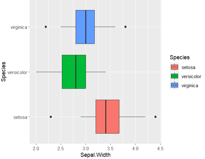
#除了反转横纵坐标之外，可使用coord_flip()改变坐标系
ggplot(data = iris,mapping = aes(x = Species, 
                                 y = Sepal.Width,
                                 fill = Species)) + 
    geom_boxplot()+
    coord_flip()

输出结果：

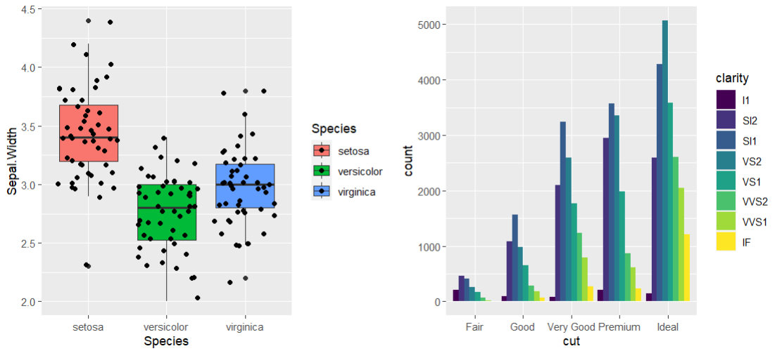
图片导出

#patchwork拼图
library(patchwork)
p1 = ggplot(data = iris,mapping = aes(x = Species, 
                                      y = Sepal.Width,
                                      fill = Species)) + 
        geom_boxplot()+
        geom_jitter()
p2 = ggplot(data = diamonds) + 
     geom_bar(mapping = aes(x = cut, fill = clarity),
              position = "dodge")
p1 + p2

#保存导出图片
#经典三段函数
pdf("data.pdf")
p1 + p2
dev.off()
#ggsave
p = p1 + p2
ggsave(p,filename = "data.png")
#eoffice
library(eoffice)
topptx(p,"data.pptx") #导出的ppt中所有图片的元素可修改

输出结果：