车辆动力学方程推导和代码实现

艰默

发布于 2024-01-23 18:45:10

2431

发布于 2024-01-23 18:45:10

文章被收录于专栏：iDoitnowiDoitnow

1. 车辆动力学模型

车辆动力学模型是描述汽车运动规律的微分方程，一般用于分析汽车的平顺性和操纵稳定性。二自由度的车辆动力学模型基于单车模型假设，只考虑轮胎侧偏特性，其应用前提是

忽略轮胎力的纵横向耦合关系。
不考虑载荷的左右转移。
忽略悬架运动、路面坡度和横纵向空气动力学等非线性效应。

2. 车辆动力学建模

由于车辆动力学模型忽略了空气动力学和地面坡度等因素，因此汽车受到的外力均来自轮胎受到的地面力，其模型的几何结构和受力分析如下图所示：

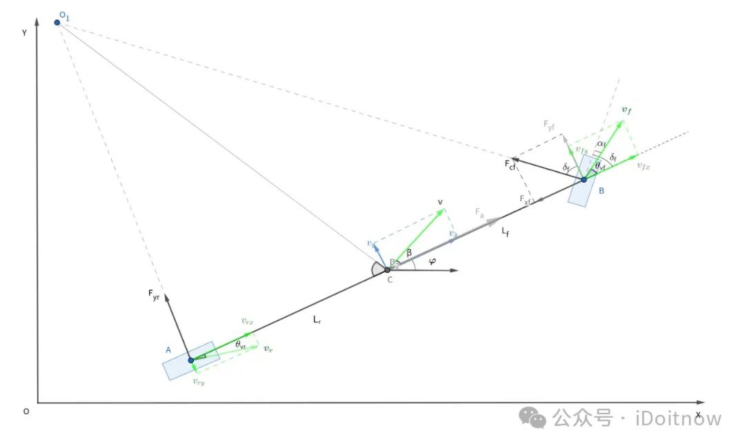
其中：

：质心

处的速度，即车辆的速度。

v_x

：质心速度

在纵向的分量。

v_y

：质心速度

在横向的分量。

v_f

：前轮的速度。

v_{fx}

：前轮的速度

v_f

在纵向的分量。

v_{fy}

：前轮的速度

v_f

在横向的分量。

v_r

：后轮的速度。

v_{rx}

：后轮的速度

v_r

在纵向的分量。

v_{ry}

：后轮的速度

v_r

在横向的分量。

\beta

：质心侧偏角度，质心速度与车辆纵向的夹角。

\varphi

：横摆角，即车辆轴线(纵向)与X轴的夹角。

：质心。

L_f

：质心到前轴的距离。

L_r

：质心到后轴的距离。

\delta_f

：前轮转角，即前轮朝向与车身纵向的夹角。

\theta_{vf}

：前轮速度偏角度（一般是由于轮胎形变引起的），即前轮速度

v_f

与车身纵向夹角。

\alpha_f

：前轮侧偏角，即前轮速度

v_f

与前轮朝向的夹角。

\delta_r

：后轮转角，我们的模型是后轮不转向，因此

\delta_r=0

，图中未标注。

\theta_{vr}

：后轮速度偏角，即后轮速度

v_r

与车身纵向夹角。

\alpha_r

：后轮侧偏角，即后轮速度

v_r

与后轮朝向的夹角，图中未标注。

F_{yf}

：前轮受到的横向力。

F_{xf}

：前轮受到的纵向力。

F_{yr}

：后轮受到的横向力。

F_{cf}

：前轮侧向力。

F_{cr}

：后轮侧向力。

忽略地面坡度，沿着车身

轴（横向）应用牛顿第二定律可得

ma_y=F_{yf}+F_{yr} \tag{1}

为车辆的质量，

a_y

为车辆在质心

处横向的惯性加速度，其主要由横向加速度

\ddot{y}

和向心加速度

v_x\dot{\varphi}

组成，即

a_y=\ddot{y}+v_x\dot{\varphi} \tag{2}

将(2)代入(1)可得

m(\ddot{y}+v_x\dot{\varphi} ) = F_{yf}+F_{yr} \tag{3}

同理，沿着车身

轴（纵向）可得

a_x = \dot{v_x}-v_y\dot{\varphi} \tag{4}

m(\dot{v_x}-v_y\dot{\varphi} )= F_a- F_{xf} \tag{5}

其中

F_a

为车辆动力系统提供的纵向力。

车辆的横向运动并不是完全的侧向平移，而是需要通过一定程度的转向来完成，也就是横摆运动，由车辆绕

轴的旋转平衡可以得到车辆的的横摆动力学方程

I_z\ddot{\varphi}=L_fF_{yf}-L_rF_{yr} \tag{6}

其中

I_z

为车辆绕

轴的转动惯量，

\ddot{\varphi}

为横摆角的加速度。

由图中角的几何关系，可得前轮侧偏角

\alpha_f = \delta_f - \theta_{vf} \tag{7}

后轮侧偏角

\alpha_r=-\theta_{vr} \tag{8}

由于轮胎在侧偏角较小的时候，轮胎的侧向力与侧偏角近似成正比，因此有

F_{cf}=C_{\alpha f}(\delta_f-\theta_{vf})\tag{9}

F_{cr} = C_{\alpha r}(-\theta_{vr}) \tag{10}

C_{\alpha f}

为前轮侧向力与前轮侧偏角的比例系数，称为前轮轮胎的侧扁刚度，

C_{\alpha r}

为后轮侧向力与后轮侧偏角的比例系数，即后轮轮胎的侧扁刚度。

注：这里推导没有乘以2，是因为我们是将车辆看作是一个两轮的自行车模型，

C_{\alpha f}

和

C_{\alpha r}

分别可以理解为两个前轮的侧扁刚度和，以及两个后轮的侧扁刚度和，在实际应用中，需要根据车辆的实际情况作适当的调整。后面的代码仿真中，我们在设置

C_{\alpha f}

和

C_{\alpha r}

的时候，会自动将其乘以2，来表示两个前轮侧扁刚度和和两个后轮侧扁刚度和。

由图中力的几何关系可得

F_{xf} = F_{cf}sin\delta_f=C_{\alpha f}(\delta_f-\theta_{vf})sin\delta_f \tag{11}

F_{yf} = F_{cf}cos\delta_f=C_{\alpha f}(\delta_f-\theta_{vf})cos\delta_f \tag{12}

F_{yr} = F_{cr} = C_{\alpha r}(-\theta_{vr}) \tag{13}

由于前后轮的横向速度由车辆自身横向速度和绕质心的转动速度组成，因此

v_{fy}=\dot{y}+L_f\dot{\varphi} \tag{14}

v_{ry}=\dot{y}-L_r \dot{\varphi} \tag{15}

其中

\dot{y}

为车辆横向速度，

\dot{\varphi}

为车辆的向心速度。

由于前后轮的纵向速度和车辆自身的纵向速度相等，即

v_{fx} = v_{rx} = v_x

，结合图中的几何关系可得

tan\theta_{vf} = \frac{v_{fy}}{v_{fx}}= \frac{\dot{y}+L_f\dot{\varphi}}{v_{x}} \tag{16}

tan\theta_{vr} = \frac{v_{ry}}{v_{rx}}= \frac{\dot{y}-L_r \dot{\varphi}}{v_{x}} \tag{17}

由(16)和(17)可得

\theta_{vf} = arctan{\frac{\dot{y}+L_f\dot{\varphi}}{v_{x}}} \tag{18}

\theta_{vr} = arctan{\frac{\dot{y}-L_r \dot{\varphi}}{v_{x}}} \tag{19}

将(18)和(19)代入到(11)、(12)和(13)可得

F_{xf} = C_{\alpha f}(\delta_f-arctan{\frac{\dot{y}+L_f\dot{\varphi}}{v_{x}}})sin\delta_f \tag{20}

F_{yf}=C_{\alpha f}(\delta_f-arctan{\frac{\dot{y}+L_f\dot{\varphi}}{v_{x}}})cos\delta_f \tag{21}

F_{yr}= C_{\alpha r}(-arctan{\frac{\dot{y}-L_r \dot{\varphi}}{v_{x}}}) \tag{22}

由(5)可得纵向加速度

\dot{v_x}

等于

\dot{v_x}=\frac{F_a- F_{xf}}{m}+v_y\dot{\varphi} \tag{23}

由(3)可得横向加速度

\dot{v_y}

等于

\dot{v_y}=\ddot{y}=\frac{F_{yf}+F_{yr}}{m}-v_x \dot{\varphi} \tag{24}

由(6)可得

\ddot{\varphi}=\frac{L_fF_{yf}-L_rF_{yr}}{I_z} \tag{25}

另外对于全局坐标

\dot{X}

和

\dot{Y}

类似坐标的旋转，所以有

\dot{X}=v_xcos\varphi-v_ysin\varphi \tag{26}

\dot{Y}=v_xsin\varphi+v_ycos\varphi \tag{27}

综上可得

\begin{cases} \dot{v_x}=a-\frac{ F_{xf}}{m}+v_y\dot{\varphi}\\ \dot{v_y}=\frac{F_{yf}+F_{yr}}{m}-v_x \dot{\varphi}\\ \ddot{\varphi}=\frac{L_fF_{yf}-L_rF_{yr}}{I_z}\\ \dot{X}=v_xcos\varphi-v_ysin\varphi \\ \dot{Y}=v_xsin\varphi+v_ycos\varphi \end{cases} \tag{28}

其中

\begin{cases} F_{xf} = C_{\alpha f}(\delta_f-\theta_{vf})sin\delta_f \\ F_{yf}=C_{\alpha f}(\delta_f-arctan{\frac{\dot{y}+L_f\dot{\varphi}}{v_{x}}})cos\delta_f\\ F_{yr}= C_{\alpha r}(-arctan{\frac{\dot{y}-L_r \dot{\varphi}}{v_{x}}}) \end{cases} \tag{29}

3. 模型实现

import math
import matplotlib.pyplot as plt
import numpy as np
# import imageio


# 车辆参数信息
L = 2.9                     # 轴距[m]
Lf = L / 2.0                # 车辆中心点到前轴的距离[m]
Lr = L - Lf                 # 车辆终点到后轴的距离[m]
W = 2.0                     # 宽度[m]
LF = 3.8                    # 后轴中心到车头距离[m]
LB = 0.8                    # 后轴中心到车尾距离[m]
TR = 0.5                    # 轮子半径[m]
TW = 0.5                    # 轮子宽度[m]
WD = W                      # 轮距[m]
Iz = 2250.0                 # 车辆绕z轴的转动惯量[kg/m2]
Cf = 1600.0 * 2.0           # 前轮侧偏刚度[N/rad]
Cr = 1700.0 * 2.0           # 后轮侧偏刚度[N/rad]
m = 1500.0                  # 车身质量[kg]
LENGTH = LB + LF            # 车辆长度[m]
MWA = np.radians(30.0)      # 最大轮转角(Max Wheel Angle)[rad]


def normalize_angle(angle):
    a = math.fmod(angle + np.pi, 2 * np.pi)
    if a < 0.0:
        a += (2.0 * np.pi)
    return a - np.pi


class DynamicBicycleModel:

    def __init__(self, x=0.0, y=0.0, yaw=0.0, vx=0.01, vy=0.0, omega=0.0):
        self.x = x
        self.y = y
        self.yaw = yaw
        self.vx = vx
        self.vy = vy
        self.omega = omega
        self.delta = 0.0

    def update(self, a, delta, dt=0.1):
        self.delta = np.clip(delta, -MWA, MWA)
        self.x = self.x + self.vx * math.cos(self.yaw) * dt - self.vy * math.sin(self.yaw) * dt
        self.y = self.y + self.vx * math.sin(self.yaw) * dt + self.vy * math.cos(self.yaw) * dt
        self.yaw = self.yaw + self.omega * dt
        self.yaw = normalize_angle(self.yaw)
        f_cf = Cf * normalize_angle(self.delta - math.atan2((self.vy + Lf * self.omega) / self.vx, 1.0))
        f_cr = Cr * math.atan2((Lr * self.omega-self.vy) / self.vx, 1.0)
        f_xf = f_cf * math.sin(self.delta)
        f_yf = f_cf * math.cos(self.delta)
        f_yr = f_cr
        self.vx = self.vx + (a - f_xf / m + self.vy * self.omega) * dt
        self.vy = self.vy + ((f_yr + f_yf) / m - self.vx * self.omega) * dt
        self.omega = self.omega + (Lf * f_yf - f_yr * Lr) / Iz * dt


def draw_vehicle(x, y, yaw, delta, ax, color='black'):
    vehicle_outline = np.array(
        [[-LB, LF, LF, -LB, -LB],
         [W / 2, W / 2, -W / 2, -W / 2, W / 2]])

    wheel = np.array([[-TR, TR, TR, -TR, -TR],
                      [TW / 2, TW / 2, -TW / 2, -TW / 2, TW / 2]])

    rr_wheel = wheel.copy()  # 右后轮
    rl_wheel = wheel.copy()  # 左后轮
    fr_wheel = wheel.copy()  # 右前轮
    fl_wheel = wheel.copy()  # 左前轮
    rr_wheel[1, :] += WD/2
    rl_wheel[1, :] -= WD/2

    # 方向盘旋转
    rot1 = np.array([[np.cos(delta), -np.sin(delta)],
                     [np.sin(delta), np.cos(delta)]])
    # yaw旋转矩阵
    rot2 = np.array([[np.cos(yaw), -np.sin(yaw)],
                     [np.sin(yaw), np.cos(yaw)]])
    fr_wheel = np.dot(rot1, fr_wheel)
    fl_wheel = np.dot(rot1, fl_wheel)
    fr_wheel += np.array([[L], [-WD / 2]])
    fl_wheel += np.array([[L], [WD / 2]])

    fr_wheel = np.dot(rot2, fr_wheel)
    fr_wheel[0, :] += x
    fr_wheel[1, :] += y
    fl_wheel = np.dot(rot2, fl_wheel)
    fl_wheel[0, :] += x
    fl_wheel[1, :] += y
    rr_wheel = np.dot(rot2, rr_wheel)
    rr_wheel[0, :] += x
    rr_wheel[1, :] += y
    rl_wheel = np.dot(rot2, rl_wheel)
    rl_wheel[0, :] += x
    rl_wheel[1, :] += y
    vehicle_outline = np.dot(rot2, vehicle_outline)
    vehicle_outline[0, :] += x
    vehicle_outline[1, :] += y

    ax.plot(fr_wheel[0, :], fr_wheel[1, :], color)
    ax.plot(rr_wheel[0, :], rr_wheel[1, :], color)
    ax.plot(fl_wheel[0, :], fl_wheel[1, :], color)
    ax.plot(rl_wheel[0, :], rl_wheel[1, :], color)

    ax.plot(vehicle_outline[0, :], vehicle_outline[1, :], color)
    # ax.axis('equal')


if __name__ == "__main__":

    vehicle = DynamicBicycleModel(0.0, 0.0, 0.0, 1.0, 1.0, 0.0)
    trajectory_x = []
    trajectory_y = []
    fig = plt.figure()

    # 保存动图用
    # i = 0
    # image_list = []  # 存储图片
    plt.figure(1)
    for i in range(500):
        plt.cla()
        plt.gca().set_aspect('equal', adjustable='box')
        vehicle.update(0, np.pi / 10)
        draw_vehicle(vehicle.x, vehicle.y, vehicle.yaw, vehicle.delta, plt)
        trajectory_x.append(vehicle.x)
        trajectory_y.append(vehicle.y)
        plt.plot(trajectory_x, trajectory_y, 'blue')
        plt.xlim(-15, 12)
        plt.ylim(-2.5, 21)
        plt.pause(0.001)
    #     i += 1
    #     if (i % 5) == 0:
    #         plt.savefig("temp.png")
    #         image_list.append(imageio.imread("temp.png"))
    #
    # imageio.mimsave("display.gif", image_list, duration=0.1)

运行效果：