文章MSM_metagenomics(四):Beta多样性分析
原创
文章MSM_metagenomics(四):Beta多样性分析
原创
生信学习者
发布于 2024-06-16 08:34:38
发布于 2024-06-16 08:34:38
欢迎大家关注全网生信学习者系列:
- WX公zhong号:生信学习者
- Xiao hong书:生信学习者
- 知hu:生信学习者
- CDSN:生信学习者2
介绍
本教程旨在使用基于R的函数以及Python脚本来估计使用MetaPhlAn profile的微生物群落的Beta多样性
数据
大家通过以下链接下载数据:
- 百度网盘链接:https://pan.baidu.com/s/1f1SyyvRfpNVO3sLYEblz1A
- 提取码: 请关注WX公zhong号生信学习者后台发送 复现msm 获取提取码
基于R的方法
R 包
Beta diversity analysis, visualization and significance assessment
使用beta_diversity_funcs.R计算alpha多样性和可视化。
- 代码
generate_coordis_df <- function(mat, md, dist_method = "bray") {
  # mat: the loaded matrix from mpa-style dataframe.
  # md: the dataframe containing metadata.
  # dist_method: the method for calculating beta diversity. default: ["bray"]. For other method, refer to vegdist()
  # this function is to prepare metadata-added coordinates dataframe.

  bray_dist <- vegan::vegdist(mat, dist_method)
  coordinates <- as.data.frame(ape::pcoa(bray_dist)$vectors)
  coor_df <- cbind(coordinates, md)

  return(coor_df)
}

pcoa_plot <- function(
  mat,
  md,
  dist_method,
  ariable,
  fsize = 11,
  dsize = 1,
  fstyle = "Arial",
  to_rm = NULL) {

  # mat: the loaded matrix from mpa-style dataframe, [dataframe].
  # md: the dataframe containing metadata, [dataframe].
  # dist_method: the method for calculating beta diversity, [string]. default: ["bray"]. For other method, refer to vegdist().
  # fsize: the font size, [int].
  # dsize: the dot size, [int].
  # fstyle: the font style, [string].
  # variable: specify the variable name for separating groups, [string].
  # to_rm: a vector of values in "variable" column where the corresponding rows will be removed first.
  # this function is to draw pcoa plot with confidence ellipse
  coordis_df <- generate_coordis_df(mat, md, dist_method)
  if (is.null(to_rm)) {
    coordis_df <- coordis_df[!(is.na(coordis_df[, variable]) | coordis_df[, variable] == ""), ]
  } else {
    coordis_df <- coordis_df[!(is.na(coordis_df[, variable]) | coordis_df[, variable] == "" | coordis_df[, variable] %in% to_rm), ]
  }

  eval(substitute(ggplot(coordis_df, aes(Axis.1, Axis.2, color = c)),list(c = as.name(variable)))) +
    geom_point(size = dsize) +
    theme_bw() +
    eval(substitute(geom_polygon(stat = "ellipse", aes(fill = c), alpha = 0.1), list(c = as.name(variable)))) +
    labs(x = "PC1", y = "PC2") +
    theme(text = element_text(size = fsize, family = fstyle)) +
    theme(legend.position="bottom")
}

est_permanova <- function(
  mat,
  md,
  variable,
  covariables = NULL,
  nper = 999,
  to_rm = NULL,
  by_method = "margin"){

  # mat: the loaded matrix from mpa-style dataframe, [dataframe].
  # md: the dataframe containing metadata, [dataframe].
  # variable: specify the variable for testing, [string].
  # covariables: give a vector of covariables for adjustment, [vector].
  # nper: the number of permutation, [int], default: [999].
  # to_rm: a vector of values in "variable" column where the corresponding rows will be removed first.
  # by_method: "terms" will assess significance for each term, sequentially; "margin" will assess the marginal effects of the terms.

  if (is.null(to_rm)) {
    clean_md <- md[!(is.na(md[, variable]) | md[, variable] == ""), ]
  } else {
    clean_md <- md[!(is.na(md[, variable]) | md[, variable] == "" | md[, variable] %in% to_rm), ]
  }
  clean_idx = rownames(clean_md)
  clean_mat <- mat[rownames(mat) %in% clean_idx, ]
  if (is.null(covariables)) {
    est <- eval(substitute(adonis2(mat ~ cat, data = md, permutations = nper, by = by_method), list(cat = as.name(variable))))
  } else {
    mat_char <- deparse(substitute(mat))
    str1 <- paste0(c(variable, paste0(covariables, collapse = " + ")), collapse = " + ")
    str2 <- paste0(c(mat_char, str1), collapse = " ~ ")
    est <- vegan::adonis2(eval(parse(text = str2)), data = md, permutations = nper, by = by_method)
  }

  return(est)
}

pcoa_sideplot <- function(
  coordinate_df,
  variable,
  color_palettes = ggpubr::get_palette(palette = "default", k = length(unique(coordinate_df[, variable]))),
  coordinate_1 = "PC1",
  coordinate_2 = "PC2",
  marker_size = 3,
  font_size = 20,
  font_style = "Arial"){

  # coordinate_df: the coordinate table generated from python script multi_variable_pcoa_plot.py --df_opt
  # variable: specify the variable you want to inspect on PCoA.
  # color_palettes: give a named vector to pair color palettes with variable group names. default: [ggpubr default palette]
  # coordinate_1: specify the column header of the 1st coordinate. default: [PC1]
  # coordinate_2: specify the column header of the 2nd coordinate. default: [PC2]
  # marker_size: specify the marker size of the PCoA plot. default: [3]
  # font_size: specify the font size of PCoA labels and tick labels. default: [20]
  # font_style: specify the font style of PCoA labels and tick labels. default: ["Arial"]

  main_plot <- ggplot2::ggplot(coordinate_df,
                               ggplot2::aes(x = .data[[coordinate_1]], y = .data[[coordinate_2]],
                                  color = .data[[variable]])) +
                               ggplot2::geom_point(size = marker_size) +
                               ggplot2::theme_bw() +
                               ggplot2::theme(text = ggplot2::element_text(size = font_size, family = font_style)) +
                               ggpubr::color_palette(color_palettes)

  xdens <- cowplot::axis_canvas(main_plot, axis = "x") +
            ggplot2::geom_density(data = coordinate_df,
                                ggplot2::aes(x = .data[[coordinate_1]], fill = .data[[variable]]),
                                alpha = 0.7,
                                size = 0.2) +
            ggpubr::fill_palette(color_palettes)

  ydens <- cowplot::axis_canvas(main_plot, axis = "y", coord_flip = TRUE) +
            ggplot2::geom_density(data = coordinate_df,
                                ggplot2::aes(x = .data[[coordinate_2]], fill = .data[[variable]]),
                                alpha = 0.7,
                                size = 0.2) +
            ggplot2::coord_flip() +
            ggpubr::fill_palette(color_palettes)

  plot1 <- cowplot::insert_xaxis_grob(main_plot, xdens, grid::unit(.2, "null"), position = "top")
  plot2 <- cowplot::insert_yaxis_grob(plot1, ydens, grid::unit(.2, "null"), position = "right")

  comb_plot <- cowplot::ggdraw(plot2)

  return(comb_plot)
}Beta多样性分析、可视化和显著性评估。加载一个由MetaPhlAn量化的物种相对丰度的矩阵表matrix table以及一个与矩阵表逐行匹配的元数据表metadata table,即在矩阵表和元数据表中,每一行都表示一个样本。
matrix <- read.csv("./data/matrix_species_relab.tsv", header = TRUE, sep = "\t")

metadata <- read.csv("./data/metadata_of_matrix_species_relab.tsv", header = TRUE, sep = "\t")现在,在调整诸如BMI和疾病状态等协变量的同时,测试样本因感兴趣的变量而分离的显著性。在这里,我们使用est_permanova函数来执行PERMANOVA分析,并指定参数:
mat: the loaded matrix from metaphlan-style table, [dataframe].md: the metadata table pairing with the matrix, [dataframe].variable: specify the variable for testing, [string].covariables: give a vector of covariables for adjustment, [vector].nper: the number of permutation, [int], default: [999].to_rm: a vector of values in "variable" column where the corresponding rows will be removed first.by_method: "terms" will assess significance for each term, sequentially; "margin" will assess the marginal effects of the terms.
在这里,我们通过一个示例来展示,在调整可能解释肠道微生物组成个体间变异的因素,包括antibiotics use, HIV status, BMI, Diet 和 Inflamatory bowel diseases等协变量的同时,测试变量condom use的显著性。
est_permanova(
    mat = matrix,
    md = metadata,
    variable = "condom_use",
    covariables = c("Antibiotics_6mo", "HIV_status", "inflammatory_bowel_disease", "BMI_kg_m2_WHO", "diet"),
    nper = 999,
    to_rm = c("no_receptive_anal_intercourse"),
    by_method = "margin")

                           Df SumOfSqs      R2      F Pr(>F)
condom_use                  4   1.2161 0.08194 1.5789  0.008 **
Antibiotics_6mo             2   0.4869 0.03281 1.2643  0.160
HIV_status                  1   0.3686 0.02484 1.9146  0.030 *
inflammatory_bowel_disease  1   0.2990 0.02015 1.5529  0.066 .
BMI_kg_m2_WHO               5   1.8376 0.12382 1.9087  0.002 **
diet                        3   0.8579 0.05781 1.4853  0.036 *
Residual                   49   9.4347 0.63571
Total                      65  14.8412 1.00000
---
Signif. codes: 0 ‘***’ 0.001 ‘**’ 0.01 ‘*’ 0.05 ‘.’ 0.1 ‘ ’ 1接下来,为了根据微生物群落的Beta多样性可视化样本的分离情况,我们可以使用plot_pcoa函数,该函数需要输入参数:
mat: the loaded matrix from metaphlan-style table, [dataframe].md: the metadata table pairing with the matrix, [dataframe].dist_method: the method for calculating beta diversity, [string]. default: ["bray"]. For other methods, refer to vegdist().fsize: the font size of labels, [int]. default: [11]dsize: the dot size of scatter plot, [int]. default: [3]fstyle: the font style, [string]. default: ["Arial"]variable: specify the variable name based on which to group samples, [string].to_rm: a vector of values in "variable" column where the corresponding rows will be excluded first before analysis.
下面,我们将展示如何从五个不同变量的角度检查微生物群落的Beta多样性。
pcoa_condom_use <- pcoa_plot(
    mat = matrix,
    md = metadata,
    dist_method = "bray",
    fsize = 11,
    dsize = 3,
    fstyle = "Arial",
    variable = "condom_use",
    to_rm = c("no_receptive_anal_intercourse"))

pcoa_STI <- pcoa_plot(
    mat = matrix,
    md = metadata,
    dist_method = "bray",
    fsize = 11,
    dsize = 3,
    fstyle = "Arial",
    variable = "STI")

pcoa_number_of_partners <- pcoa_plot(
    mat = matrix,
    md = metadata,
    dist_method = "bray",
    fsize = 11,
    dsize = 3,
    fstyle = "Arial",
    variable = "number_partners")

pcoa_rai <- pcoa_plot(
    mat = matrix,
    md = metadata,
    dist_method = "bray",
    fsize = 11,
    dsize = 3,
    fstyle = "Arial",
    variable = "receptive_anal_intercourse")

pcoa_oral_sex <- pcoa_plot(
    mat = matrix,
    md = metadata,
    dist_method = "bray",
    fsize = 11,
    dsize = 3,
    fstyle = "Arial",
    variable = "oral.sex")

pcoa_lubricant_use <- pcoa_plot(
    mat = matrix,
    md = metadata,
    dist_method = "bray",
    fsize = 11,
    dsize = 3,
    fstyle = "Arial",
    variable = "lubricant")

ggarrange(pcoa_rai, pcoa_lubricant_use, pcoa_STI,
          pcoa_oral_sex, pcoa_number_of_partners, pcoa_condom_use,
nrow = 2, ncol = 3) 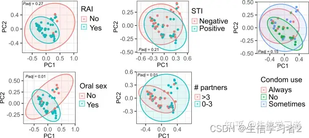
基于Python的办法
Python 包
Beta diversity analysis with PCoA plotting integrating maximum three variables
multi_variable_pcoa_plot.py 用于做PCoA分析
- 代码和用法
#!/usr/bin/env python

"""
NAME: multi_variable_pcoa_plot.py
DESCRIPTION: multi_variable_pcoa_plot.py is a python script to perform principal coordinate analysis based on
             taxanomic abundance or functional abundances with the possibility of analyzing three parameters together.
             Of note, multi_variable_pcoa_plot can be used as module too.
"""

from skbio.diversity import beta_diversity
from skbio.stats.ordination import pcoa
from skbio.stats.distance import DistanceMatrix
import pandas as pd
import numpy as np
import matplotlib.pyplot as plt
import matplotlib
import seaborn as sns
import sys
import argparse
import math
from skbio.stats.distance import anosim
import textwrap
from collections import namedtuple

def read_args(args):
    # This function is to parse arguments

    parser = argparse.ArgumentParser(formatter_class=argparse.RawDescriptionHelpFormatter,
                                    description = textwrap.dedent('''\
                                     This program is to do PCoA analysis on microbial taxonomic or functional abundance data integrating maximum three variables together.
                                     '''),
                                    epilog = textwrap.dedent('''\
                                    examples:
                                    pcoa_painter.py --abundance_table <merged_metaphlan_table> --metadata <metadata> --sample_column <sample_header> --variable1 <variable1_name> --variable2 <variable2_name> --variable3 <variable3_name> --output_figure <output.png>
                                    '''))

    parser.add_argument('--abundance_table',
                        nargs = '?',
                        help = 'Input the merged abundance table generated by MetaPhlAn.',
                        type = str,
                        default = None)

    parser.add_argument('--metadata',
                        nargs = '?',
                        help = 'Input a tab-delimited metadata file.',
                        type = str,
                        default = None)

    parser.add_argument('--transformation',
                        nargs = '?',
                        help = 'Specify the tranformation function applied on data points in the original table. \
                                For abundance table, you can choose <sqrt>/<log>. \
                                Default setting is <None>.',
                        type = str,
                        default = None)

    parser.add_argument('--metric',
                        nargs = '?',
                        help = 'Specify the metric you want to use for calculating beta diversity in the case of as input using \
                                abundance table.<braycurtis>/<unweighted_unifrac>/<jaccard>/<weighted_unifrac>. \
                                Default setting is <braycurtis>',
                        type = str,
                        default = 'braycurtis')

    parser.add_argument('--amplifier',
                        nargs = '?',
                        help = 'Specify how much you want to amplify your original data point. For example, \
                        <--amplifier 100> indicates that all original data point times 100. Default is 1.',
                        type = int,
                        default = 1)

    parser.add_argument('--sample_column',
                        nargs = '?',
                        help = 'Specify the header of column containing metagenome sample names in the metadata file.',
                        type = str,
                        default = None)

    parser.add_argument('--variable1',
                        nargs = '?',
                        help = 'Specify the header of the variable in the metadata table you want to assess. This variable will be represented by colors.',
                        type = str,
                        default = None)

    parser.add_argument('--variable2',
                        nargs = '?',
                        help = 'Specify the header of second variable in the metadata table you want to assess. This variable will be represented by marker shapes.',
                        type = str,
                        default = None)

    parser.add_argument('--variable3',
                        nargs = '?',
                        help = 'Specify the header of the third variable in the metadata table you want to assess. This variable will be represented by marker sizes.',
                        type = str,
                        default = None)

    parser.add_argument('--marker_palette',
                        nargs = '?',
                        help = 'Input a tab-delimited mapping file where 1st column contains group names and 2nd column contains color codes. default: [None] (automatic handling)',
                        type = str,
                        default = None)

    parser.add_argument('--marker_shapes',
                        nargs = '?',
                        help = 'Input a tab-delimited mapping file where 1st column contains group names and 2nd column contains marker shapes. default: [None] (automatic handling)',
                        type = str,
                        default = None)

    parser.add_argument('--marker_sizes',
                        nargs = '?',
                        help = 'Input a tab-delimited mapping file where values are group names and keys are marker size. default: [None] (automatic handling)',
                        type = str,
                        default = None)

    parser.add_argument('--output_figure',
                        nargs = '?',
                        help = 'Specify the name for the output figure. For example, output_figure.svg',
                        type = str,
                        default = None)

    parser.add_argument('--test',
                        nargs = '?',
                        help = 'Specify an output file for saving permanova test results. For example, project_name_stats.tsv',
                        type = str,
                        default = None)


    parser.add_argument('--df_opt',
                        nargs = '?',
                        help = 'Specify the output name for saving coordinates (PC1 and PC2) for each sample. For example, project_name_coordinates.tsv',
                        type = str,
                        default = None)

    parser.add_argument('--font_style',
                        nargs = '?',
                        help = 'Specify the font style which is composed by font family and font type, delimited with a comma. default: [sans-serif,Arial]',
                        type = str,
                        default = "sans-serif,Arial")

    parser.add_argument('--font_size',
                        nargs = '?',
                        help = 'Specify the font size. default: [11]',
                        type = int,
                        default = 11)

    return vars(parser.parse_args())

class BetaDiversity:

    """
    This object is to deal with beta diversity analysis
    """

    def __init__(self, matrix_value, metadata):
        # matrix_value: the merged standard relative abundance table from metaphlan.
        # metadata: the tab-delimited metadata file, each column contains one metadata parameter.

        self.abundance_table = matrix_value
        self.metadata = metadata

    def est_beta_diversity_matrix(self, trans_func, diversity_metric, amplifier):
        # trans_func: the function for transforming abundance values, e.g. sqrt or log.
        # diversity_metric: the metric for calculating beta diversity, e.g. jaccard or braycurtis.
        # amplifier: N times the relative abundnce values, e.g. 10000
        # this function is to estimate beta diversity by users' defined transformation function and metric.

        raw_df = pd.read_csv(self.abundance_table, sep = "\t", index_col = False) # read merged metaphlan table into a dataframe
        df = raw_df.loc[(raw_df.sum(axis=1) != 0), (raw_df.sum(axis=0) != 0)] # clean raw df by removing zero-sum rows and columns
        ids = df.columns[1:] # get all sample names
        matrix = [] # the matrix of rel abundance, each row contains all abundances for one sample
        for s in ids:
            bug_abundances_one_sample = []
            for i in df.index:
                abundance_value = df.loc[i, s]
                if trans_func == None:
                    bug_abundances_one_sample.append(float(abundance_value) * amplifier)
                elif trans_func == 'sqrt':
                    bug_abundances_one_sample.append(math.sqrt(float(abundance_value) * amplifier))
                elif trans_func == 'log':
                    bug_abundances_one_sample.append(math.log1p(float(abundance_value) * amplifier + 1))
                else:
                    sys.exit("Please choose transformation function from <sqrt>/<log>/<None>")
            matrix.append(bug_abundances_one_sample)

        return beta_diversity(diversity_metric, matrix, ids)
    def get_valid_samples(self):
        # this function is to return a list of valid samples to match with metadata.
        raw_df = pd.read_csv(self.abundance_table, sep = "\t", index_col = False)
        df = raw_df.loc[(raw_df.sum(axis=1) != 0), (raw_df.sum(axis=0) != 0)]

        return df.columns

    def get_valid_metadata(self, index_col, variables):
        # index_col: the column name for index column.
        # variable: the variable parameter one wants to map on the PCoA plot.
        variables = [i for i in variables if i]
        variables = list(set(variables))
        if len(variables) > 0:
            metadata_df = pd.read_csv(self.metadata, sep = "\t", index_col = index_col)[variables]
            valid_samples = self.get_valid_samples() # get all samples which match with those in the metadata table.
            metadata_index = metadata_df.index
            rows_to_drop = [i for i in metadata_index if i not in valid_samples]
            metadata_df = metadata_df.drop(rows_to_drop) # drop those rows in the metadata table where samples cannot be found in the abundance table
            return metadata_df
        else:
            sys.exit("None of three variables were detected. Please specify at least one variable using --variable1, --variable2 or --variable3!")

    def pcoa_df(self, data_matrix, index_col, variables):
        # data_matrix: the skbio style matrix fed into PCoA analysis.
        # index_col: the column name for index column.
        # variable: the variable parameter one wants to map on the PCoA plot.
        # this function is to perform pcoa analysis on the skbio-style matrix.
        variables = [i for i in variables if i ]
        variables = list(set(variables))
        if len(variables) > 0:
            PCoAs= pcoa(data_matrix)
            coordinates= PCoAs.samples.loc[:, ["PC1", "PC2"]] # Take first two coordinates
            PC_explained = PCoAs.proportion_explained
            PC1_p = round(PC_explained['PC1']*100,2) #PC1 explained percentage
            PC2_p = round(PC_explained['PC2']*100,2) #PC2 explained percentage
            metadata_df = self.get_valid_metadata(index_col, variables)
            return pd.concat([coordinates, metadata_df], axis = 1), PC1_p, PC2_p
        else:
            sys.exit("None of three variables were detected. Please specify at least one variable using --variable1, --variable2 or --variable3!")


    def permanova_test(self, data_matrix, index_col, variable):
        # data_matrix: the skbio style matrix fed into PCoA analysis.
        # this function is to perform permanova test.
        # Note: this test is a bit inconsistent with R package, be careful.

        permanova_results = namedtuple('permanova_results', ['statistic', 'pvalue'])

        metadata_df = self.get_valid_metadata(index_col, [variable])

        anosim_test = anosim(data_matrix, metadata_df, column= variable, permutations = 999)


        return permanova_results(anosim_test['test statistic'], anosim_test["p-value"])

    def pcoa_plotting(self, data_matrix, opt_figure, index_col, df_opt,
                      variable1 = None, variable2 = None, variable3 = None,
                      marker_sizes = None, marker_palette = None, marker_shapes = None,
                      font_style = "sans-serif,Arial", font_size = 11):
        # this function is to plot the PCoA analysis results
        # palette: a mapping file in which 1st column is group name and 2nd column is color code. No header row!
        font_family, font_type = font_style.split(",")
        fig, ax = plt.subplots()
        matplotlib.rcParams['font.family'] = font_family
        matplotlib.rcParams['font.{}'.format(font_family)] = font_type
        variables = [variable1, variable2, variable3]
        pcoa_coords, PC1_p, PC2_p = self.pcoa_df(data_matrix, index_col, variables)
        if marker_palette:
            palette_dict = {i.rstrip().split('\t')[0]: i.rstrip().split('\t')[1] for i in open(marker_palette).readlines()}
        else:
            palette_dict = None

        if marker_shapes:
            shape_dict = {i.rstrip().split('\t')[0]: i.rstrip().split('\t')[1] for i in open(marker_shapes).readlines()}
        else:
            shape_dict = True

        if marker_sizes:
            sizes_dict = {i.rstrip().split('\t')[0]: float(i.rstrip().split('\t')[1]) for i in open(marker_sizes).readlines()}
        else:
            sizes_dict = None

        if df_opt:
            pcoa_coords.to_csv(df_opt, sep = "\t", index = False)


        sns.scatterplot(x = "PC1", y = "PC2", data = pcoa_coords,
                        hue = variable1, palette = palette_dict,
                        style = variable2,
                        markers = shape_dict,
                        size = variable3, sizes = sizes_dict,
                        ax = ax)

        ax.set_xlabel('PC1({}%)'.format(str(PC1_p)), fontsize = font_size)
        ax.tick_params(axis = "x", labelsize = font_size)
        ax.set_ylabel('PC2({}%)'.format(str(PC2_p)), fontsize = font_size)
        ax.tick_params(axis = "y", labelsize = font_size)
        ax.legend(bbox_to_anchor=(1.01, 1), loc=2,borderaxespad=0.)
        fig.savefig(opt_figure, bbox_inches = 'tight', dpi = 600)

if __name__ == '__main__':
    pars = read_args(sys.argv)
    if pars['metadata']:
        if pars['sample_column']:
            variables = list(set([pars['variable1'], pars['variable2'], pars['variable3']]))
            variables = [i for i in variables if i]
            if len(variables) > 0:
                b_diversity_analysis = BetaDiversity(pars['abundance_table'], pars['metadata'])
                b_diversity_matrix = b_diversity_analysis.est_beta_diversity_matrix(pars['transformation'],
                                                                                    pars['metric'],
                                                                                    pars['amplifier'])
                b_diversity_analysis.pcoa_plotting(b_diversity_matrix,
                                                   pars['output_figure'],
                                                   pars['sample_column'],
                                                   pars['df_opt'],
                                                   variable1 = pars['variable1'],
                                                   variable2 = pars['variable2'],
                                                   variable3 = pars['variable3'],
                                                   marker_sizes = pars['marker_sizes'],
                                                   marker_palette = pars['marker_palette'],
                                                   marker_shapes = pars['marker_shapes'],
                                                   font_style = pars['font_style'],
                                                   font_size = pars['font_size']
                                                   )
                if pars['test']:
                    results_matrix = []
                    for single_variable in variables:
                        permanova_opt = b_diversity_analysis.permanova_test(b_diversity_matrix,
                                                                             pars['sample_column'],
                                                                             single_variable)

                        results_matrix.append([single_variable, permanova_opt.statistic, permanova_opt.pvalue])
                    stats_df = pd.DataFrame(results_matrix, columns = ['factor', 'statistic', 'p-value'])
                    stats_df.to_csv(pars['test'], sep = '\t', index = False)
            else:
                sys.exit("None of three variables were detected. Please specify at least one variable using --variable1, --variable2 or --variable3!")
        else:
            sys.exit('Please specify the column name containing samples!')
    else:
sys.exit('Please input a proper metadata file!')- 用法
usage: multi_variable_pcoa_plot.py [-h] [--abundance_table [ABUNDANCE_TABLE]] [--metadata [METADATA]] [--transformation [TRANSFORMATION]] [--metric [METRIC]] [--amplifier [AMPLIFIER]] [--sample_column [SAMPLE_COLUMN]] [--variable1 [VARIABLE1]] [--variable2 [VARIABLE2]] [--variable3 [VARIABLE3]]
                                   [--marker_palette [MARKER_PALETTE]] [--marker_shapes [MARKER_SHAPES]] [--marker_sizes [MARKER_SIZES]] [--output_figure [OUTPUT_FIGURE]] [--test [TEST]] [--df_opt [DF_OPT]] [--font_style [FONT_STYLE]] [--font_size [FONT_SIZE]]

This program is to do PCoA analysis on microbial taxonomic or functional abundance data integrating maximum three variables together.

optional arguments:
  -h, --help            show this help message and exit
  --abundance_table [ABUNDANCE_TABLE]
                        Input the merged abundance table generated by MetaPhlAn.
  --metadata [METADATA]
                        Input a tab-delimited metadata file.
  --transformation [TRANSFORMATION]
                        Specify the tranformation function applied on data points in the original table. For abundance table, you can choose <sqrt>/<log>. Default setting is <None>.
  --metric [METRIC]     Specify the metric you want to use for calculating beta diversity in the case of as input using abundance table.<braycurtis>/<unweighted_unifrac>/<jaccard>/<weighted_unifrac>. Default setting is <braycurtis>
  --amplifier [AMPLIFIER]
                        Specify how much you want to amplify your original data point. For example, <--amplifier 100> indicates that all original data point times 100. Default is 1.
  --sample_column [SAMPLE_COLUMN]
                        Specify the header of column containing metagenome sample names in the metadata file.
  --variable1 [VARIABLE1]
                        Specify the header of the variable in the metadata table you want to assess. This variable will be represented by colors.
  --variable2 [VARIABLE2]
                        Specify the header of second variable in the metadata table you want to assess. This variable will be represented by marker shapes.
  --variable3 [VARIABLE3]
                        Specify the header of the third variable in the metadata table you want to assess. This variable will be represented by marker sizes.
  --marker_palette [MARKER_PALETTE]
                        Input a tab-delimited mapping file where 1st column contains group names and 2nd column contains color codes. default: [None] (automatic handling)
  --marker_shapes [MARKER_SHAPES]
                        Input a tab-delimited mapping file where 1st column contains group names and 2nd column contains marker shapes. default: [None] (automatic handling)
  --marker_sizes [MARKER_SIZES]
                        Input a tab-delimited mapping file where values are group names and keys are marker size. default: [None] (automatic handling)
  --output_figure [OUTPUT_FIGURE]
                        Specify the name for the output figure. For example, output_figure.svg
  --test [TEST]         Specify an output file for saving permanova test results. For example, project_name
  --df_opt [DF_OPT]     Specify the output name for saving coordinates (PC1 and PC2) for each sample. For example, project_name_coordinates.tsv
  --font_style [FONT_STYLE]
                        Specify the font style which is composed by font family and font type, delimited with a comma. default: [sans-serif,Arial]
  --font_size [FONT_SIZE]
                        Specify the font size. default: [11]

examples:

python multi_variable_pcoa_plot.py --abundance_table <merged_metaphlan_table> --metadata <metadata> --sample_column <sample_header> --variable1 <variable1_name> --variable2 <variable2_name> --variable3 <variable3_name> --output_figure <output.png>为了演示multi_variable_pcoa_plot.py的使用,我们将根据来自11个人群的样本微生物组成绘制一个PCoA图,这些人群被分为 W (Westernization), NW (Non-Westernization), NWU (Non-Westernization(Urban)) 和 MSM (Men-having-sex-with-men)。不同的人群将使用自定义颜色,通过颜色映射文件color map file: ./data/mvpp_color_map.tsv进行分配,而MSM人群将通过标记大小映射文件marker size map file: ./data/mvpp_marker_size_map.tsv使用更大的标记大小来突出显示。每个样本的元数据由元数据文件metadata file: ./data/mvpp_metadata.tsv提供。
示例命令:
python multi_variable_pcoa_plot.py \
  --abundance_table mvpp_mpa_species_relab.tsv \
  --metadata mvpp_metadata.tsv \
  --sample_column sample \
  --variable1 country \
  --variable2 westernization \
  --variable3 country \
  --output_figure mvpp_pcoa.png \
  --test mvpp_permanova.tsv \
  --df_opt mvpp_coordinates_df.tsv \
  --marker_palette mvpp_color_map.tsv \
  --marker_sizes mvpp_marker_size_map.tsv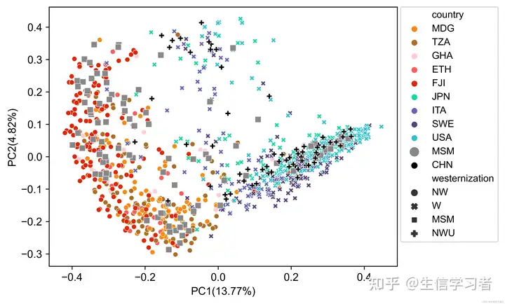
作为可选输出,get_palette(palette = "default", k) 还生成了非调整的PERMANOVA测试结果(例如 mvpp_permanova.tsv: ./data/mvpp_permanova.tsv)以及PC1和PC2的坐标(例如 mvpp_coordinates.tsv: ./data/mvpp_coordinates.tsv)。
A method mixing R and Python
R packages required
Beta diversity analysis with PCoA plotting using pre-calculated coordinates
如果您希望使用R增强PCoA图的美观性,但使用multi_variable_pcoa_plot.py预计算的坐标,并带有标志--df_opt,建议您使用我们的R函数pcoa_sideplot(),该函数作用于multi_variable_pcoa_plot.py的坐标表,并带有参数
coordinate_df: the coordinate table generated from python script multi_variable_pcoa_plot.py --df_opt, for example coordinate_table.tsv: ./data/coordinate_table.tsv.variable: specify the variable you want to inspect on PCoA.color_palettes: give a named vector to pair color palettes with variable group names. default: [ggpubr default palette]coordinate_1: specify the column header of the 1st coordinate. default: [PC1]coordinate_2: specify the column header of the 2nd coordinate. default: [PC2]marker_size: specify the marker size of the PCoA plot. default: [3]font_size: specify the font size of PCoA labels and tick labels. default: [20]font_style: specify the font style of PCoA labels and tick labels. default: [Arial]
比如:
coordinate_df <- data.frame(read.csv("./data/coordinate_table.tsv", header = TRUE, sep = "\t"))
pcoa_sideplot(coordinate_df = coordinate,
              coordinate_1 = "PC1",
              coordinate_2 = "PC2",
              variable = "sexual_orientation",
              color_palettes = c("Non-MSM" = "#888888", "MSM" = "#eb2525"))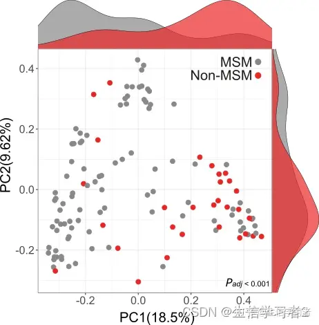
原创声明:本文系作者授权腾讯云开发者社区发表,未经许可,不得转载。
如有侵权,请联系 cloudcommunity@tencent.com 删除。
原创声明:本文系作者授权腾讯云开发者社区发表,未经许可,不得转载。
如有侵权,请联系 cloudcommunity@tencent.com 删除。
评论
登录后参与评论
推荐阅读
目录
腾讯云开发者

Copyright © 2013 - 2026 Tencent Cloud. All Rights Reserved. 腾讯云 版权所有
深圳市腾讯计算机系统有限公司 ICP备案/许可证号:粤B2-20090059 ![]() 粤公网安备44030502008569号
粤公网安备44030502008569号
腾讯云计算(北京)有限责任公司 京ICP证150476号 | 京ICP备11018762号