单细胞实战之cellchat——入门到进阶(高级篇1）

原创

凑齐六个字吧

发布于 2025-04-13 16:32:24

2.8K0

文章被收录于专栏：单细胞单细胞

在中级篇中已经完成了细胞亚群的细分流程，并回顾了几个重要的分析工具。接下来将进入高级篇的内容。首先将回顾最常用的细胞通讯工具之一——CellChat。在该讲中会按照单一及两样本进行分析。

本次内容涉及到的工程文件可通过网盘获得：中级篇2，链接: https://pan.baidu.com/s/1y-HHLXoXsJbgWKCdz26-gQ 提取码: yx93 ；初级篇2 链接: https://pan.baidu.com/s/1ETVEkJNCJSe9NU7_aLEPVA 提取码: znmb 。

此外，可以向“生信技能树”公众号发送关键词‘单细胞’，直接获取Seurat V5版本的完整代码。

Cellchat简介

Cellchat能够从scRNA-seq数据中定量推断和分析细胞间通讯网络，其预测细胞的主要信号的输入及输出，以及这些细胞和信号是如何通过网络分析和模式识别方法进行协调从而执行功能。Cellchat中配体-受体分析主要基于质量作用定律模型量化两个细胞群体之间的信号通讯概率，其中的质量作用定律模型是指形成复合物的速率（即信号强度）与配体和受体的浓度有关。

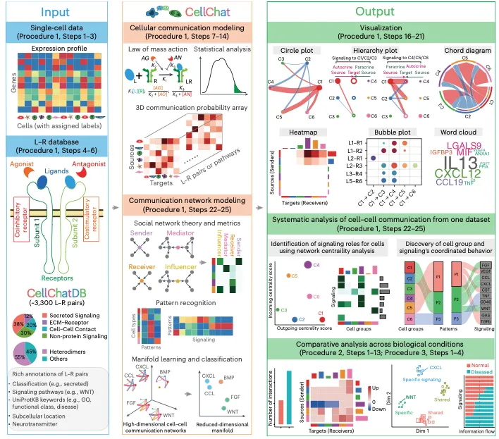
研究团队构建了一个专用于分析细胞间信号连接的数据库——CellChatDB。该数据库全面整合了配体、受体及其辅助因子之间的相互作用信息，考虑了配体–受体复合物的已知结构形式，同时纳入了多种辅助因子，如可溶性的激动剂、拮抗剂，以及具有共刺激性或共抑制性的膜结合受体。CellChatDB融合了来自KEGG数据库的信号分子相互作用信息，以及文献中已有实验证实的配体–受体组合，为系统分析细胞通信提供了坚实的数据基础。在cellchat V2版中共包含3300条已验证的分子相互作用，其中39.6%为旁分泌/自分泌信号，13.1%为细胞外基质-受体相互作用，16.5%为细胞接触相关相互作用，约30%为非蛋白质信号传导。

Cellchat细胞通讯分析的主要内容如下：

为了预测显著的通讯，CellChat识别出每个细胞组中差异过表达的配体和受体。为了量化由这些信号基因介导的两个细胞组之间的通讯，CellChat将每个相互作用与一个概率值相关联。后者是基于配体在一个细胞组中的平均表达值和受体在另一个细胞组中的平均表达值，以及它们的协同因子。

配体-受体相互作用：每个细胞类型都会表达特定的配体和受体。细胞通讯分析通过研究这些配体和受体之间的相互作用，来了解细胞是如何“交流”的。例如，一个细胞释放的配体可以与另一种细胞的受体结合，从而触发一系列细胞内的信号传导事件。
信号通路活性：通过分析相互作用在不同细胞类型之间进行作用，研究者可以了解哪些信号通路在特定生物学过程中起作用，如细胞分化、免疫反应或疾病状态等。
细胞间网络构建：细胞通讯分析通常会构建一个细胞间的网络图，显示不同细胞类型之间的相互作用方式。这个网络可以帮助识别主要的信号发送者和接收者，以及哪些细胞在组织中起主导作用。
定量分析：通过计算细胞通讯的强度（如配体-受体结合的概率），可以定量分析不同细胞类型之间的通讯强度。这可以揭示在特定条件下，哪种细胞类型在通讯中占主导地位。
功能富集分析：细胞通讯分析还可以与功能富集分析结合使用，探讨哪些生物学功能或通路受到特定细胞通讯的调控。

CellChat 相较于其他工具，如 SingleCellSignalR、iTALK 和 NicheNet，具有显著优势，它考虑了许多受体作为多亚基复合物存在的情况。此外，虽然 CellPhoneDB v2.0 能够通过异源复合物成员的最小平均表达来预测两个细胞群体之间的富集信号相互作用，但它未能纳入其他关键的信号辅助因子，如可溶性激动剂、拮抗剂，以及具有刺激性或抑制性的膜结合共受体。除此之外，CellChat 还具备强大的可视化输出功能，有助于更直观地进行数据解释和分析。

单样本Cellchat分析流程

1.导入

rm(list = ls())
library(Matrix)
library(CellChat) # 2.1.2版本
library(qs)
library(Seurat)
library(patchwork)
library(BiocParallel)
register(MulticoreParam(workers = 8, progressbar = TRUE))
sub_data <- qread("./9-CD4+T/CD4+t_final.qs")
scRNA <- qread("./4-Corrective-data/sce.all.qs")

dir.create("./13-cellchat")
setwd("./13-cellchat")

2.数据预处理

把细分亚群整合到原来的数据集中，但需要提醒一件事，在CD4+T细胞分群的时候清洗了很多细胞，因此CD8+T和NK等一些细胞亚群在既往是没有保存的！！但如果是做科研、讲“故事”，请务必要把所有细分亚群统统保存下来，纳入一起分析！！

# check一下
p1 <- DimPlot(sub_data,pt.size = 0.8,group.by = "celltype",label = T)
p2 <- DimPlot(scRNA,pt.size = 0.8,group.by = "celltype",label = T)
p1|p2

table(scRNA@meta.data$celltype)
phe <- scRNA@meta.data
table(sub_data@meta.data$celltype)
phe_t <- sub_data@meta.data
# 找到匹配的行索引
matched_indices <- match(rownames(phe), rownames(phe_t))
# 根据匹配的行，phe_t$celltype的值赋给phe$status
phe$celltype[!is.na(matched_indices)] <- phe_t$celltype[matched_indices[!is.na(matched_indices)]]
table(phe$celltype)
scRNA@meta.data <- phe
table(scRNA$celltype)
Idents(scRNA) <- scRNA$celltype
DimPlot(scRNA,label = F)

# CellChat需要两个用户输入:一个是细胞的基因表达数据，另一个是用户分配的细胞标签。
# 对于基因表达数据矩阵，行为基因，列为细胞。
# CellChat需要数据归一化数据。如果是count数据，使用normalizeData进行归一化。
# 本次数据已经进行过归一化处理了

3.创建Cellchat对象

data.input <- GetAssayData(scRNA, slot = 'data') # normalized data matrix
meta <- scRNA@meta.data[,c("orig.ident","celltype")]
colnames(meta) <-  c("group","labels")
table(meta$labels)
meta$labels <- gsub(" cells", "", meta$labels)
#meta$labels <- sub("\\(.*\\)", "", meta$labels)
table(meta$labels)

identical(rownames(meta),colnames(data.input))
## 根据研究情况进行细胞排序
celltype_order <- c(
  "T/NK", 
  "Th1", 
  "Th17", 
  "Tm", 
  "Treg", 
  "Naive T", 
  "ELK4+T", 
  "ZNF793+T", 
  "ZSCAN12+T",
  "B", 
  "VSMCs", 
  "endothelial", 
  "epithelial/cancer", 
  "fibroblasts", 
  "mast", 
  "myeloid", 
  "plasma", 
  "proliferative"
)
meta$labels <- factor(meta$labels ,levels = celltype_order)
table(meta$labels)

# 根据 meta$labels 的顺序进行排序
ordered_indices <- order(meta$labels)
# 对 meta 和 data.input 进行排序
meta <- meta[ordered_indices, ]
data.input <- data.input[, ordered_indices]
identical(rownames(meta),colnames(data.input))

# 构建cellchat
cellchat <- createCellChat(object = data.input, meta = meta, group.by = "labels")
levels(cellchat@idents)
#  [1] "T/NK"              "Th1"               "Th17"              "Tm"                "Treg"             
#  [6] "Naive T"           "ELK4+T"            "ZNF793+T"          "ZSCAN12+T"         "B"                
# [11] "VSMCs"             "endothelial"       "epithelial/cancer" "fibroblasts"       "mast"             
# [16] "myeloid"           "plasma"            "proliferative"

4.设置配体-受体相互作用数据库

研究者不建议把非蛋白质信号纳入分析，这可能是由于在单细胞转录组数据中无法准确检测或量化、对应的信号分子不直接由基因编码，而是代谢产物、离子等、生物学机制复杂，且缺乏统一可靠的注释和数据库支持等原因。

CellChatDB <- CellChatDB.human # use CellChatDB.mouse if running on mouse data
showDatabaseCategory(CellChatDB)
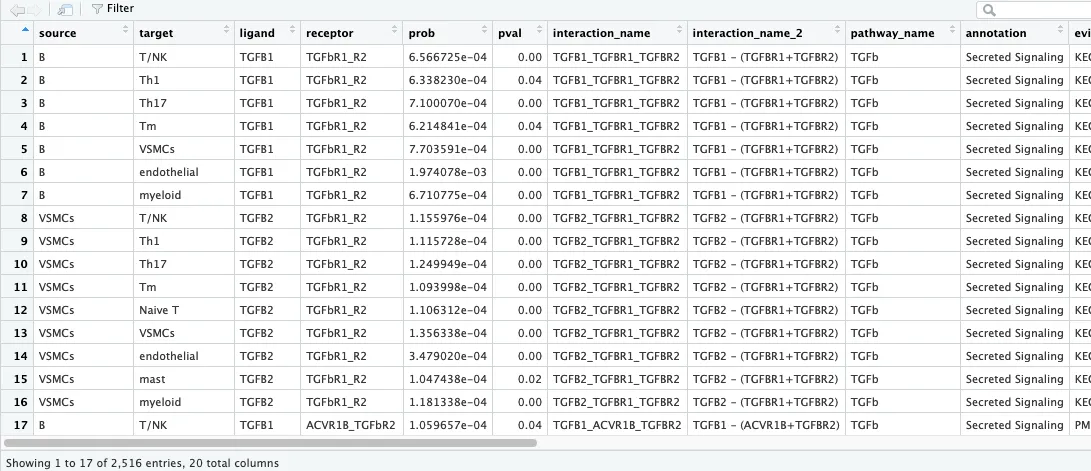
dplyr::glimpse(CellChatDB$interaction)
# Rows: 3,234
# Columns: 28
# $ interaction_name         <chr> "TGFB1_TGFBR1_TGFBR2", "TGFB2_TGFBR1_TGFBR2", "TGFB3_TGFBR1_TGFBR2", "TGFB1_ACVR…
# $ pathway_name             <chr> "TGFb", "TGFb", "TGFb", "TGFb", "TGFb", "TGFb", "TGFb", "TGFb", "TGFb", "TGFb", …
# $ ligand                   <chr> "TGFB1", "TGFB2", "TGFB3", "TGFB1", "TGFB1", "TGFB2", "TGFB2", "TGFB3", "TGFB3",…
# $ receptor                 <chr> "TGFbR1_R2", "TGFbR1_R2", "TGFbR1_R2", "ACVR1B_TGFbR2", "ACVR1C_TGFbR2", "ACVR1B…
# $ agonist                  <chr> "TGFb agonist", "TGFb agonist", "TGFb agonist", "TGFb agonist", "TGFb agonist", …
# $ antagonist               <chr> "TGFb antagonist", "TGFb antagonist", "TGFb antagonist", "TGFb antagonist", "TGF…
# $ co_A_receptor            <chr> "", "", "", "", "", "", "", "", "", "", "", "", "", "", "", "", "", "", "", "", …
# $ co_I_receptor            <chr> "TGFb inhibition receptor", "TGFb inhibition receptor", "TGFb inhibition recepto…
# $ evidence                 <chr> "KEGG: hsa04350", "KEGG: hsa04350", "KEGG: hsa04350", "PMID: 27449815
        
        IF: 6.9 Q1 B2", "PMID: 2…
# $ annotation               <chr> "Secreted Signaling", "Secreted Signaling", "Secreted Signaling", "Secreted Sign…
# $ interaction_name_2       <chr> "TGFB1 - (TGFBR1+TGFBR2)", "TGFB2 - (TGFBR1+TGFBR2)", "TGFB3 - (TGFBR1+TGFBR2)",…
# $ is_neurotransmitter      <lgl> FALSE, FALSE, FALSE, FALSE, FALSE, FALSE, FALSE, FALSE, FALSE, FALSE, FALSE, FAL…
# $ ligand.symbol            <chr> "TGFB1", "TGFB2", "TGFB3", "TGFB1", "TGFB1", "TGFB2", "TGFB2", "TGFB3", "TGFB3",…
# $ ligand.family            <chr> "TGF-beta", "TGF-beta", "TGF-beta", "TGF-beta", "TGF-beta", "TGF-beta", "TGF-bet…
# $ ligand.location          <chr> "Extracellular matrix, Secreted, Extracellular space", "Extracellular matrix, Se…
# $ ligand.keyword           <chr> "Disease variant, Signal, Reference proteome, Extracellular matrix, Disulfide bo…
# $ ligand.secreted_type     <chr> "growth factor", "growth factor", "cytokine;growth factor", "growth factor", "gr…
# $ ligand.transmembrane     <lgl> FALSE, FALSE, TRUE, FALSE, FALSE, FALSE, FALSE, TRUE, TRUE, FALSE, FALSE, TRUE, …
# $ receptor.symbol          <chr> "TGFBR2, TGFBR1", "TGFBR2, TGFBR1", "TGFBR2, TGFBR1", "TGFBR2, ACVR1B", "TGFBR2,…
# $ receptor.family          <chr> "Protein kinase superfamily, TKL Ser/Thr protein kinase", "Protein kinase superf…
# $ receptor.location        <chr> "Cell membrane, Secreted, Membrane raft, Cell surface, Cell junction, Tight junc…
# $ receptor.keyword         <chr> "Membrane, Secreted, Disulfide bond, Kinase, Transmembrane, Differentiation, ATP…
# $ receptor.surfaceome_main <chr> "Receptors", "Receptors", "Receptors", "Receptors", "Receptors", "Receptors", "R…
# $ receptor.surfaceome_sub  <chr> "Act.TGFB;Kinase", "Act.TGFB;Kinase", "Act.TGFB;Kinase", "Act.TGFB;Kinase", "Act…
# $ receptor.adhesome        <chr> "", "", "", "", "", "", "", "", "", "", "", "", "", "", "", "", "", "", "", "", …
# $ receptor.secreted_type   <chr> "", "", "", "", "", "", "", "", "", "", "", "", "", "", "", "", "", "", "", "", …
# $ receptor.transmembrane   <lgl> TRUE, TRUE, TRUE, TRUE, TRUE, TRUE, TRUE, TRUE, TRUE, TRUE, TRUE, TRUE, TRUE, TR…
# $ version                  <chr> "CellChatDB v1", "CellChatDB v1", "CellChatDB v1", "CellChatDB v1", "CellChatDB …


# 使用CellChatDB的中特定的数据库进行细胞-细胞通信分析
# 示例中使用了Secreted Signaling
# CellChatDB.use <- subsetDB(CellChatDB, search = "Secreted Signaling", key = "annotation") 

# Only uses the Secreted Signaling from CellChatDB v1
#  CellChatDB.use <- subsetDB(CellChatDB, search = list(c("Secreted Signaling"), c("CellChatDB v1")), key = c("annotation", "version"))

# 除“非蛋白信号”外，使用所有CellChatDB数据进行细胞-细胞通信分析
CellChatDB.use <- subsetDB(CellChatDB)

# 使用所有CellChatDB数据进行细胞-细胞通信分析
# 研究者不建议以这种方式使用它，因为CellChatDB v2包含“非蛋白信号”(即代谢和突触信号)。
# CellChatDB.use <- CellChatDB 

# 在构建的cellchat中设定需要使用的数据库
cellchat@DB <- CellChatDB.use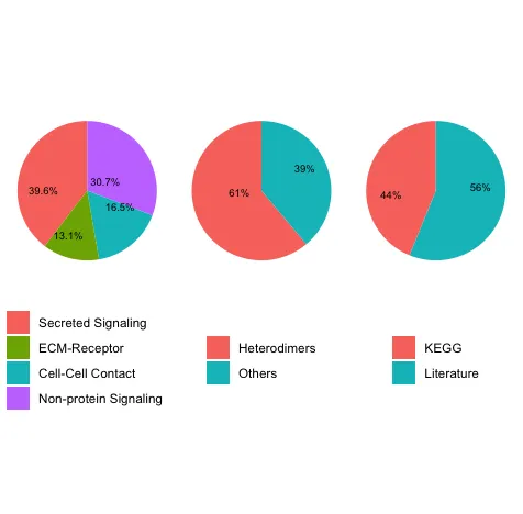

5.预处理细胞-细胞通讯分析的表达数据

cellchat <- subsetData(cellchat) # This step is necessary even if using the whole databa
future::plan("multisession", workers = 1) # do parallel
cellchat <- identifyOverExpressedGenes(cellchat)
cellchat <- identifyOverExpressedInteractions(cellchat)
#默认情况下,cellchat使用object@data.signaling进行网络推断
#同时也提供了projectData函数,通过扩散过程基于高置信度实验验证的蛋白质互作网络中的邻近节点对基因表达值进行平滑处理。该功能在处理测序深度较浅的单细胞数据时尤为有用，因其能减少信号基因（特别是配体/受体亚基可能存在的零表达）的dropout效应。不担心其可能在扩散过程引入伪影，因其仅会引发极微弱的通讯信号。
# 原来是projectData，新版是smoothData函数
cellchat <- smoothData(cellchat, adj = PPI.human)

6.细胞-细胞通信网络的推理

参数设定：‘triMean’会产生更少但更强的相互作用；而‘truncatedMean’方法中，当‘trim’参数值较小时（例如 ‘trim = 0.1或0.05’），会输出更多的相互作用，从而能够检测到较弱的信号传导活动。

# 该分析的关键参数是类型，即计算每个细胞组的平均基因表达的方法。默认情况下，type = “triMean”，产生较少但更强的交互。当设置 type = “truncatedMean” 时，应为trim分配一个值，从而产生更多交互。请详细检查上述计算每个细胞组平均基因表达的方法。
# 使用的是投射到PPI网络的模式时候需要用FALSE。如果使用了raw data就需要设置为TRUE
cellchat <- computeCommunProb(cellchat, type = "triMean",raw.use = FALSE) 

# 如果所研究的信号没有被测到，可以采用如下函数进行探查，trim设为0.1或者0.05
# computeAveExpr(cellchat, features = c("CXCL12","CXCR4"),type =  "truncatedMean",trim = 0.1)
# 如果发现修改参数之后所研究的信号被测到了，那就修改代码如下
# cellchat <- computeCommunProb(cellchat, type =  "truncatedMean",trim = 0.1,raw.use = FALSE) 

# min.cells是设置阈值，最小是需要10个细胞参与通讯推断(可以自定义)
cellchat <- filterCommunication(cellchat, min.cells = 10)

7.在信号通路水平上推断细胞间通讯

# CellChat通过汇总与每个信号通路相关的所有配体-受体相互作用的通信概率来计算信号通路水平上的通信概率。 
# NB:推断的每个配体-受体对的细胞间通信网络和每个信号通路分别存储在槽'net'和'netP'中。
cellchat <- computeCommunProbPathway(cellchat)

#数据提取，subsetCommunication函数，一般全部提取并保存
#df.net <- subsetCommunication(cellchat, sources.use = c(1,2), targets.use = c(4,5)) #表示从细胞群 1 和 2 向细胞群 4 和 5 推断出的细胞间通讯。
#df.net <- subsetCommunication(cellchat, signaling = c("WNT", "TGFb"))
df.net <- subsetCommunication(cellchat)

qsave(cellchat,"cellchat.qs")
save(df.net,file = "df.net.Rdata")
write.csv(df.net,"df.net.csv")

有了这张表格后续可以个性化的绘制很多东西

8.可视化流程

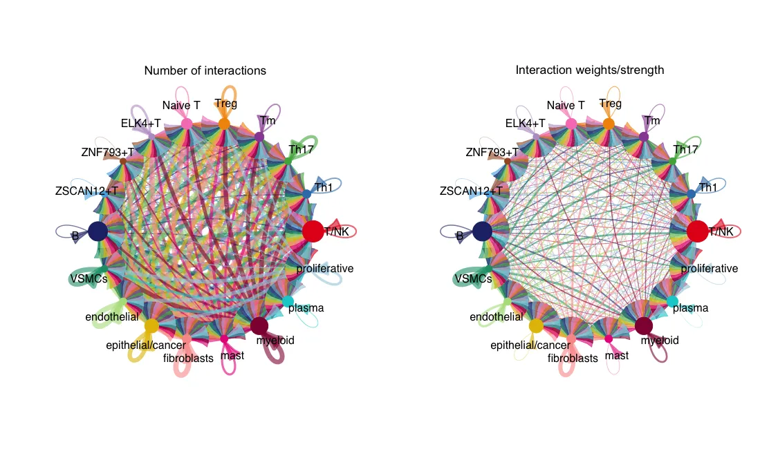
CellChat可以可视化聚合的蜂窝间通信网络。circle展示互作数目

# 计算聚合细胞-细胞通信网络
# 互作网络整合,可以设置soure和target，不设置就是默认全部
cellchat <- aggregateNet(cellchat)
# 可视化
groupSize <- as.numeric(table(cellchat@idents)) 
par(mfrow = c(1,2), xpd=TRUE)
netVisual_circle(cellchat@net$count, vertex.weight = groupSize,
                 weight.scale = T, label.edge= F, title.name = "Number of interactions")
netVisual_circle(cellchat@net$weight, vertex.weight = groupSize, 
                 weight.scale = T, label.edge= F, title.name = "Interaction weights/strength")

这两张图分别展示了互作的数量和互作的权重。其中每个颜色代表了不同的细胞，箭头代表了顺序，线的粗细代表了数量/权重。

9.heatmap展示互作数据

pheatmap::pheatmap(cellchat@net$count, border_color = "black", 
                   cluster_cols = F, fontsize = 10, cluster_rows = F,
                   display_numbers = T,number_color="black",number_format = "%.0f")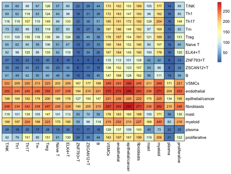

10.贝克图

展示每一个celltype作为source与其他celltype的互作情况

#指定顺序和指定颜色
celltype_order <- c(
  "T/NK",
  "Th1",
  "Th17",
  "Tm",
  "Treg",
  "Naive T",
  "ELK4+T",
  "ZNF793+T",
  "ZSCAN12+T",
  "B",
  "VSMCs",
  "endothelial",
  "epithelial/cancer",
  "fibroblasts",
  "mast",
  "myeloid",
  "plasma",
  "proliferative"
)

# 生成颜色向量（例如使用彩虹色）
color.use <- rainbow(nrow(mat))
# 将颜色向量命名为矩阵的行名
names(color.use) <- rownames(mat)
mat <- as.data.frame(cellchat@net$weight)
mat <- mat[celltype_order,]#行排序
mat <- mat[,celltype_order] %>% as.matrix()

# 如果图片显示不全,需要考虑是不是重新设置mfrow
par(mfrow = c(5,4), xpd=TRUE,mar = c(1, 1, 1, 1))
for (i in 1:nrow(mat)) {
  mat2 <- matrix(0, nrow = nrow(mat), ncol = ncol(mat), dimnames = dimnames(mat))
  mat2[i, ] <- mat[i, ]
  netVisual_circle(mat2, vertex.weight = groupSize, 
                   weight.scale = T, arrow.size=0.05,
                   arrow.width=1, edge.weight.max = max(mat), 
                   title.name = rownames(mat)[i],
                   color.use = color.use)
}

其中每个颜色代表了不同的细胞，箭头代表了顺序，线的粗细代表了数量/权重。

11.层次结构图

cellchat@netP$pathways
levels(cellchat@idents) 
pathways.show <- "CXCL"

# Hierarchy plot
# vertex.receiver定义层次图的左边细胞
vertex.receiver = seq(1:9) # a numeric vector
netVisual_aggregate(cellchat, signaling = pathways.show,
                    vertex.receiver = vertex.receiver,layout= "hierarchy")
                  # vertex.size = groupSize)  
# circle plot
netVisual_aggregate(cellchat, signaling = pathways.show,layout = "circle")

# Chord diagram
par(mfrow=c(1,1))
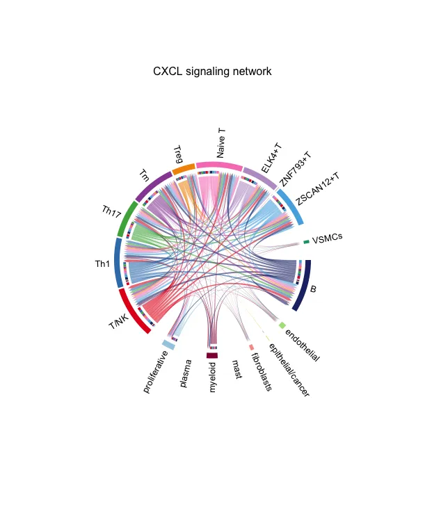
netVisual_aggregate(cellchat, signaling = pathways.show, layout = "chord")
# 分组弦图
group.cellType <- c(rep("T/NK", 9), "B","VSMCs","endothelial","epithelial/cancer",
                    "fibroblasts","mast","myeloid","plasma","proliferative" )
levels(cellchat@idents)
names(group.cellType) <- levels(cellchat@idents)
netVisual_chord_cell(cellchat, signaling = pathways.show,
                     group = group.cellType,
                     title.name = paste0(pathways.show, " signaling network"))

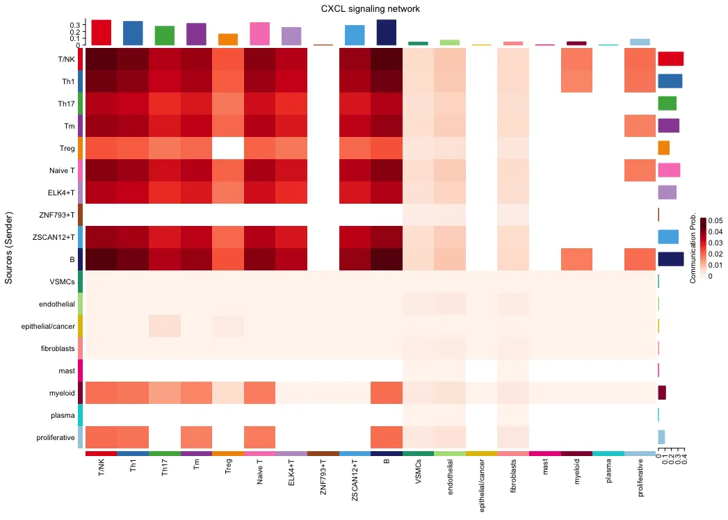
# heatmap
par(mfrow=c(1,1))
netVisual_heatmap(cellchat, signaling = pathways.show, color.heatmap = "Reds")

层次图：vertex.receiver设定了source的细胞类型(实心圆圈)，空心圆圈代表target。左半边图片先把代表vertex.receiver的圆圈放在了中间，显示了不同细胞类型对其他细胞的作用情况，右半边图片把代表其他细胞的圆圈放在了中间，显示了不同细胞类型对其余细胞的作用情况，线的粗细代表互作的强度。

Circle图和分组弦图：不同颜色代表不同细胞类型，结合箭头代表作用方向，粗细代表互作的强度，两个图很表达方式几乎一样。

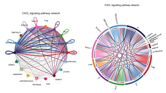
分组弦图：笔者把T细胞相关的设定成一组之后会跟其他细胞之间存在一定的分组关系

热图：

行：热图的行代表了不同的细胞类型，这些细胞作为信号的发送者。
列：热图的列代表了不同的细胞类型，这些细胞作为信号的接收者。
颜色深浅：热图中的颜色深浅表示了通讯概率的大小。颜色越深，表示通讯概率越高，这意味着发送方细胞和接收方细胞之间的信号传递越强。
通信概率（Communication Prob.）：右侧的颜色条是颜色映射的参考。图中的深红色表示较高的通讯概率（靠近0.05），浅色表示较低的通讯概率（靠近0或更低）。
顶部数值范围 (0 - 0.3)：显示不同细胞类型接受到总传入信号强度(incoming）
右侧部分的数值范围 (0 - 0.4)：显示不同细胞类型发出的总传出信号强度(outcoming）

12.计算配-受体对信号通路的贡献并可视化

# 计算配-受体对信号通路的贡献并可视化
netAnalysis_contribution(cellchat, signaling = pathways.show)

# 可视化由单个配体-受体对介导的细胞间通讯
pairLR <- extractEnrichedLR(cellchat, signaling = pathways.show,
                                 geneLR.return = FALSE)
pairLR
#   interaction_name
# 1      CXCL1_CXCR2
# 2      CXCL2_CXCR2
# 3      CXCL3_CXCR2
# 4      CXCL8_CXCR2
# 5     CXCL12_CXCR4
# 6     CXCL12_ACKR3
# 7     CXCL16_CXCR6
LR.show <- pairLR[2,] # show one ligand-receptor pair

# Hierarchy plot
vertex.receiver = seq(1,9) # a numeric vector
netVisual_individual(cellchat, signaling = pathways.show,  
                     pairLR.use = LR.show, 
                     vertex.receiver = vertex.receiver,
                     layout = "hierarchy")

# Circle plot
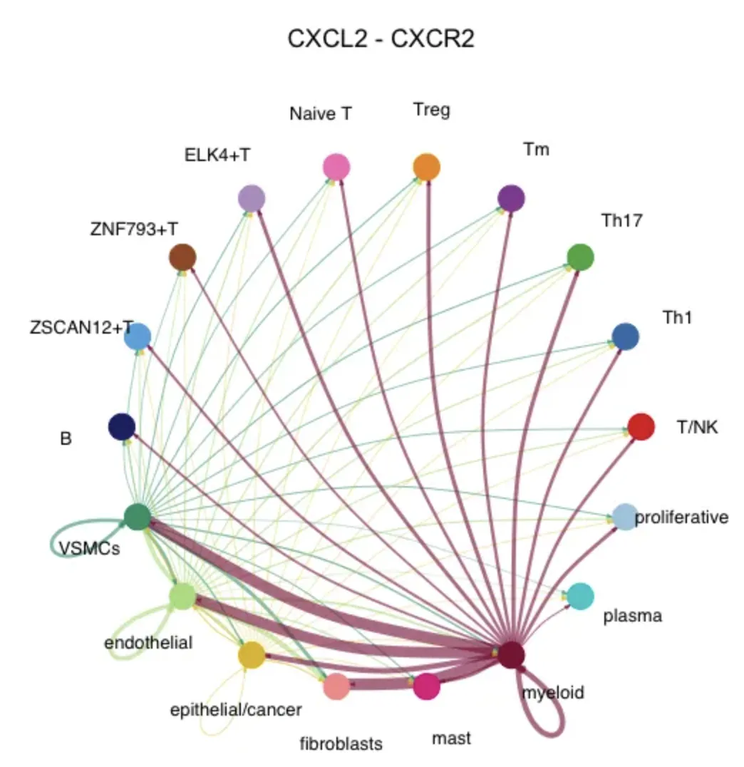
netVisual_individual(cellchat, signaling = pathways.show, 
                     pairLR.use = LR.show, layout = "circle")

展示通路下特定受配体对的贡献强度

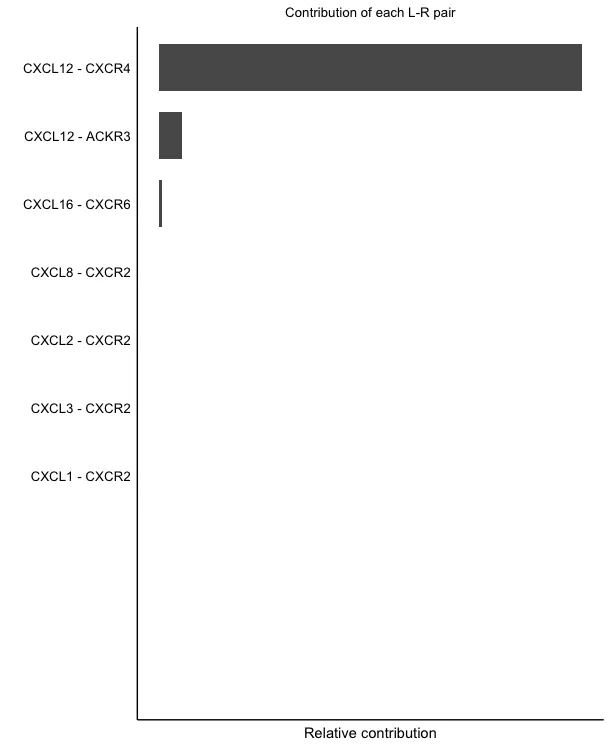
展示特定受配体对的层次图和Circle图, CXCL2-CXCR2受配体对是炎症及免疫调控中的关键信号通路，配体CXCL2主要由中性粒细胞、巨噬细胞、内皮细胞等分泌，强效的中性粒细胞趋化因子，介导炎症反应和免疫细胞募集；受体CXCR2广泛存在于中性粒细胞、单核细胞、T细胞亚群、内皮细胞及多种肿瘤细胞表面。

13.save figs

一般不这么保存

# # Access all the signaling pathways showing significant communications
# pathways.show.all <- cellchat@netP$pathways
# # check the order of cell identity to set suitable vertex.receiver
# levels(cellchat@idents)
# vertex.receiver = seq(1,3)
# for (i in 1:length(pathways.show.all)) {
#   # Visualize communication network associated with both signaling pathway and individual L-R pairs
#   netVisual(cellchat, signaling = pathways.show.all[i], vertex.receiver = vertex.receiver, layout = "hierarchy")
#   # Compute and visualize the contribution of each ligand-receptor pair to the overall signaling pathway
#   gg <- netAnalysis_contribution(cellchat, signaling = pathways.show.all[i])
#   ggsave(filename=paste0(pathways.show.all[i], "_L-R_contribution.pdf"), plot=gg, width = 3, height = 2, units = 'in', dpi = 300)
# }

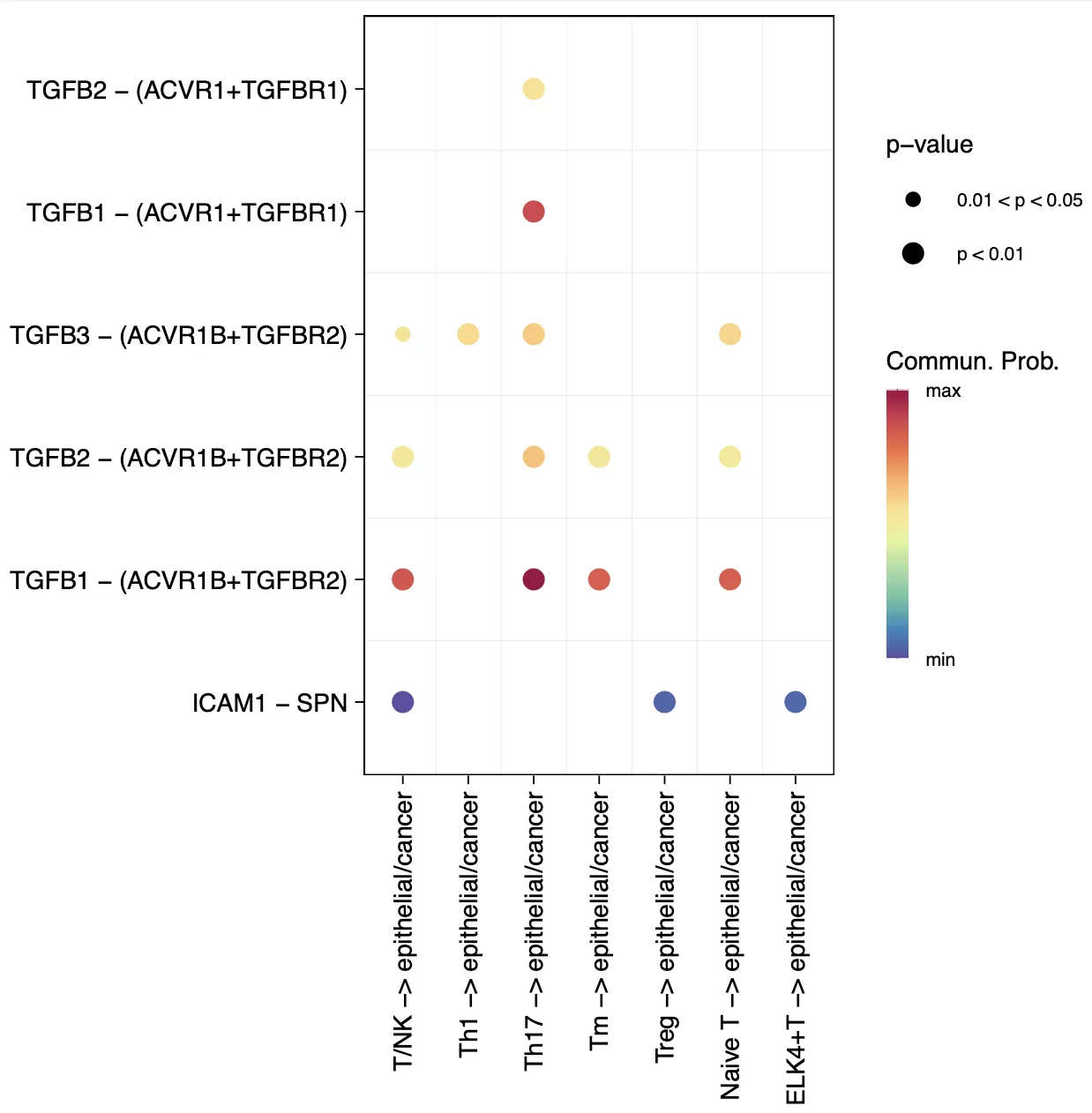
14.基于配-受体结果进一步可视化

Bubble plot, 使用netVisual_bubble显示一些单元组与其他单元组之间的所有重要相互作用

# 需要指定source和target
# sources.use是发出信号的细胞系,target.use是接受信号的细胞系
levels(cellchat@idents) 
netVisual_bubble(cellchat, sources.use = seq(1:9), 
                 targets.use = c(13), remove.isolate = FALSE)
ggsave("bubbleplot_nont.pdf",width = 7,height = 20)

# 还可以增加signaling参数用于展示特定的配受体
cellchat@netP$pathways
netVisual_bubble(cellchat, sources.use = seq(1:9), 
                 targets.use = c(13), 
                 signaling = c("CXCL"),
                 remove.isolate = FALSE)
ggsave("bubbleplot2.pdf",width = 5,height = 10)

# 自定义signaling输入展示-所有通路汇总之后
pairLR.use <- extractEnrichedLR(cellchat, signaling = c("CXCL","COLLAGEN","MK","CD99",
                                                      "LAMININ","APP","DESMOSOME"))
netVisual_bubble(cellchat, sources.use = c(1:9),
                 targets.use = c(13,14), 
                 pairLR.use = pairLR.use,
                 remove.isolate = TRUE)
ggsave("bubbleplot-LR.pdf",width = 5,height = 10)

# 可以通过增加下面的参数去设置X轴上的顺序
# sort.by.target = T
# sort.by.source = T
# sort.by.source = T, sort.by.target = T
# sort.by.source = T, sort.by.target = T, sort.by.source.priority = FALSE

不同T细胞亚群对肿瘤细胞的全部的受配体通路展示(截取部分内容)，气泡的颜色代表通讯概率大小。

不同T细胞亚群对肿瘤细胞的VEGF受配体通路展示，气泡的颜色代表通讯概率大小。

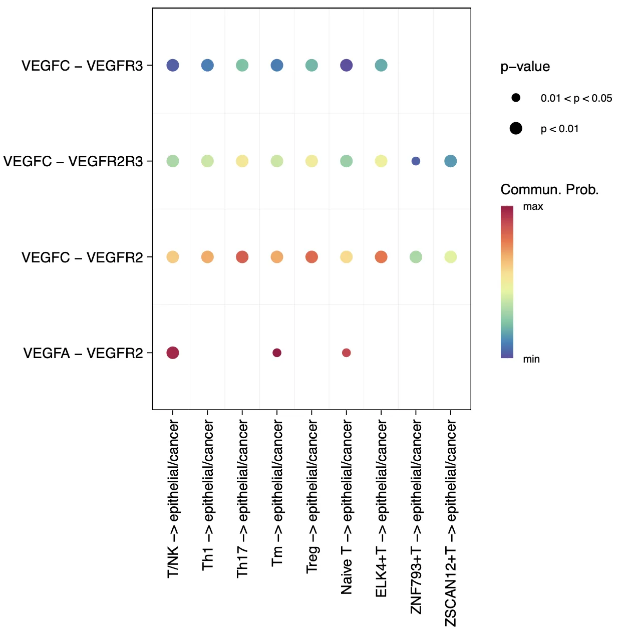
选定特定的受配体通路进行展示。

15. Chord diagram

不重复展示，结果很类似。

# 这里进行绘制时建议设定singaling或者减少互作的细胞
# 内容大多会导致不出图
cellchat@netP$pathways
netVisual_chord_gene(cellchat, sources.use = c(1:9), 
                     targets.use = c(13), 
                     signaling = c("VEGF"),
                     lab.cex = 0.5,
                     legend.pos.y = 30)

# 显示从某些细胞组(sources.use)到其他细胞组(targets.use)的所有重要信号通路。
netVisual_chord_gene(cellchat, sources.use = c(1:9), 
                     targets.use = c(13), 
                     slot.name = "netP", 
                     legend.pos.x = 10)
# NB: Please ignore the note when generating the plot such as “Note: The first link end is drawn out of sector ‘MIF’.”. If the gene names are overlapped, you can adjust the argument small.gap by decreasing the value.

16.使用小提琴/点图绘制信号转导基因表达分布

# CellChat可以使用Seurat包装函数plotGeneExpression绘制与L-R对或信号通路相关的信号转导基因的基因表达分布。
# 该功能提供 “violin”、“dot”、“bar” 三种类型的可视化。
# 或用户可以使用 extractEnrichedLR 提取与推断的 L-R 对或信号通路相关的信号转导基因，然后使用Seurat或其他软件包绘制基因表达。
plotGeneExpression(cellchat, signaling = "VEGF", 
                   enriched.only = TRUE, 
                   type = "violin")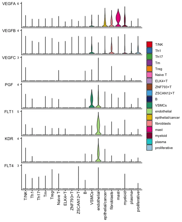

17.计算并可视化网络中心性得分

cellchat@netP$pathways
pathways.show <- "VEGF"
# Compute the network centrality scores
cellchat <- netAnalysis_computeCentrality(cellchat, 
                                          slot.name = "netP") 
netAnalysis_signalingRole_network(cellchat, signaling = pathways.show, 
                                  width = 8, height = 2.5, font.size = 10)

行（Sender, Receiver, Mediator, Influencer）：行表示在信号通路网络中，不同细胞类型扮演的角色：

Sender：信号的发送者，即哪些细胞类型是主要的信号发出者。
Receiver：信号的接收者，即哪些细胞类型是主要的信号接收者。
Mediator：中介者，用于识别在信号传播路径中起中介作用的细胞群体。
Influencer：影响者，用于识别在整个网络中对信息传播影响最大的细胞群体。列（不同的细胞类型）：列表示具体的细胞类型。颜色深浅（Importance）：颜色的深浅表示每个细胞类型在特定角色中的重要性。颜色越深，表示该细胞类型在这个角色中的重要性越高（例如信号传递的强度或频率越大）；颜色越浅，表示该细胞类型在这个角色中的重要性较低。

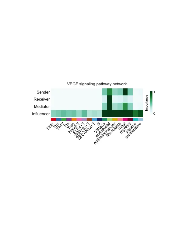
这里的分析利用了两个重要的 R 包：igraph和sna。其中，igraph包主要用于构建网络图、计算节点的出度与入度，并进行网络可视化，因其在处理加权有向图和大规模网络方面表现出色；而sna包则专注于社会网络分析，提供了流介数和信息中心度等高级网络中心性指标，这些指标有助于识别在信息传递过程中起中介作用以及对整个网络具有高度影响力的细胞群体。

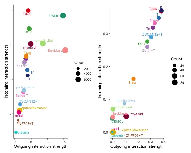
17.1 在二维空间中可视化占优势的发送者(源)和接收者(目标)

# 从所有信号通路对聚合细胞-细胞通信网络的信号作用分析
gg1 <- netAnalysis_signalingRole_scatter(cellchat);gg1
# 对特定细胞间通讯网络的信号作用分析
gg2 <- netAnalysis_signalingRole_scatter(cellchat, signaling = c("CXCL"));gg2
gg1 + gg2

左边代表所有信号的综合评估，可以看到VSMCs在输出信号方面的强度很大。右边代表特定信号的评估，这里选择了CXCL信号。可以看到B细胞在输出信号方面的强度很大。

17.2 识别对某些细胞群的输出或输入信号贡献最大的信号

# ht1 <- netAnalysis_signalingRole_heatmap(cellchat, pattern = "outgoing")
# ht1
# ht2 <- netAnalysis_signalingRole_heatmap(cellchat, pattern = "incoming")
# ht2
# ht1 + ht2
# class(ht1)

# 特定的signaling
cellchat@netP$pathways
htout <- netAnalysis_signalingRole_heatmap(cellchat, 
                                        pattern = "outgoing",
                                        signaling = c("ICAM","TGFb"))
htout

htcome <- netAnalysis_signalingRole_heatmap(cellchat, 
                                        pattern = "incoming",
                                        signaling = c("ICAM","TGFb"))
htcome

左图顶部色柱显示不同细胞的传出强度，右边色柱显示不同信号通路总传出强度。右图顶部色柱显示不同细胞的传入强度，右边色柱显著不同信号的总传入强度。

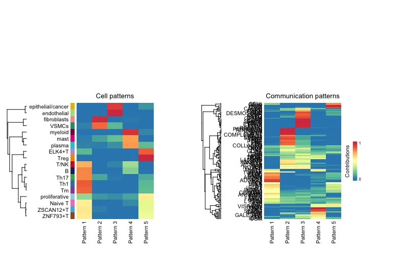
17.3 识别整体通信模式/以探索多种细胞类型和信号通路如何协调运作

outgoing

library(NMF)
library(ggalluvial)
selectK(cellchat, pattern = "outgoing")

# 当输出模式的数量为5时，Cophenetic值和Silhouette值都开始突然下降。
nPatterns = 5
cellchat <- identifyCommunicationPatterns(cellchat, 
                                          pattern = "outgoing", 
                                          k = nPatterns)
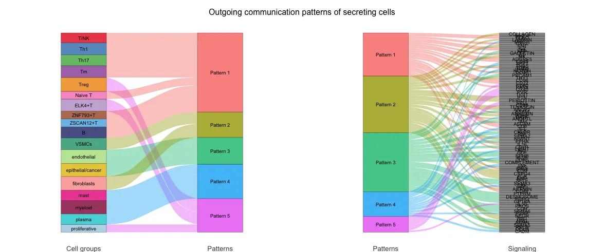
# river plot
netAnalysis_river(cellchat, pattern = "outgoing")
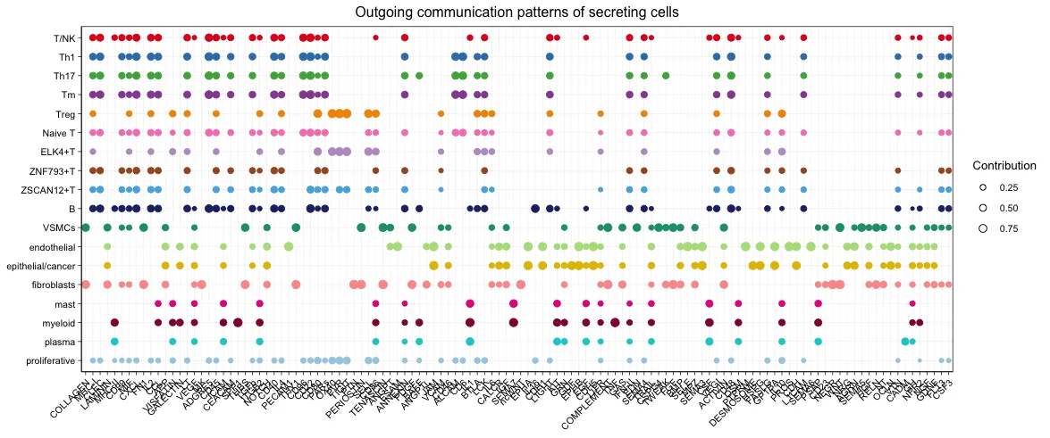
# dot plot
netAnalysis_dot(cellchat, pattern = "outgoing")

当输出模式的数量为5时，Cophenetic值和Silhouette值都开始突然下降。

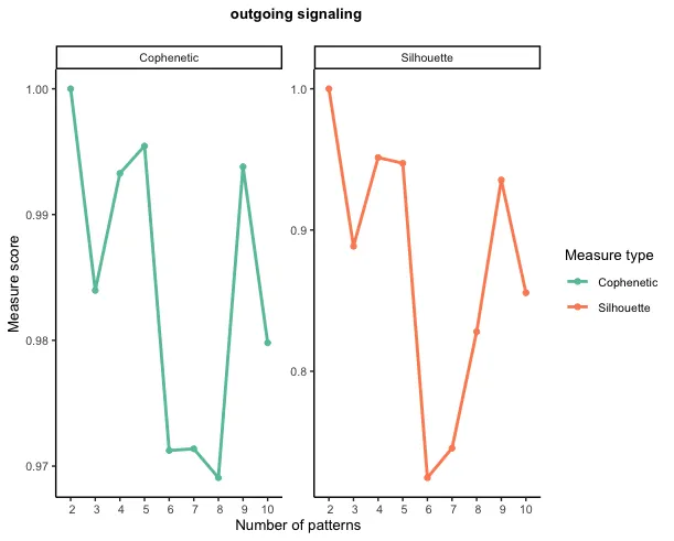
可以分成5个不同的模式，同时看到不同细胞和信号通路分别在5个模式中的贡献情况。

同上类似结果

incoming 结果不展示。

selectK(cellchat, pattern = "incoming")

# 当输出模式的数量为6时，Cophenetic值和Silhouette值都开始突然下降。
nPatterns = 6
cellchat <- identifyCommunicationPatterns(cellchat, 
                                          pattern = "incoming", 
                                          k = nPatterns)
# river plot
netAnalysis_river(cellchat, pattern = "incoming")
# dot plot
netAnalysis_dot(cellchat, pattern = "incoming")

两样本Cellchat分析流程

1.导入

rm(list = ls())
library(CellChat) # 2.1.2版本
library(Matrix)
library(qs)
library(Seurat)
library(patchwork)
library(BiocParallel)
register(MulticoreParam(workers = 8, progressbar = TRUE))
sub_data <- qread("./9-CD4+T/CD4+t_final.qs")
scRNA <- qread("./4-Corrective-data/sce.all.qs")

dir.create("./13-cellchat")
setwd("./13-cellchat")

2.数据预处理

# check一下
p1 <- DimPlot(sub_data,pt.size = 0.8,group.by = "celltype",label = T)
p2 <- DimPlot(scRNA,pt.size = 0.8,group.by = "celltype",label = T)
p1|p2

table(scRNA@meta.data$celltype)
phe <- scRNA@meta.data
table(sub_data@meta.data$celltype)
phe_t <- sub_data@meta.data
# 找到匹配的行索引
matched_indices <- match(rownames(phe), rownames(phe_t))
# 根据匹配的行，phe_t$celltype的值赋给phe$status
phe$celltype[!is.na(matched_indices)] <- phe_t$celltype[matched_indices[!is.na(matched_indices)]]
table(phe$celltype)
scRNA@meta.data <- phe
table(scRNA$celltype)
Idents(scRNA) <- scRNA$celltype
DimPlot(scRNA,label = F)

# CellChat需要两个用户输入:一个是细胞的基因表达数据，另一个是用户分配的细胞标签。
# 对于基因表达数据矩阵，行为基因，列为细胞。
# CellChat需要数据归一化数据。如果是count数据，使用normalizeData进行归一化。
# 本次数据已经进行过归一化处理了

# 拆分数据
scRNA_left <- scRNA[,scRNA$location%in% c("left")]
scRNA_right <-scRNA[,scRNA$location%in% c("right")]
# check
DimPlot(scRNA_left)|DimPlot(scRNA_right)

3.分别创建Cellchat对象

cellchat_left

# 自己分析的时候记得改名，这里是scRNA_left
data.input <- GetAssayData(scRNA_left, slot = 'data') # normalized data matrix
meta <- scRNA_left@meta.data[,c("orig.ident","celltype")]
colnames(meta) <-  c("group","labels")
table(meta$labels)
meta$labels <- gsub(" cells", "", meta$labels)
#meta$labels <- sub("\\(.*\\)", "", meta$labels)
table(meta$labels)

identical(rownames(meta),colnames(data.input))
## 根据研究情况进行细胞排序
celltype_order <- c(
  "T/NK", 
  "Th1", 
  "Th17", 
  "Tm", 
  "Treg", 
  "Naive T", 
  "ELK4+T", 
  "ZNF793+T", 
  "ZSCAN12+T",
  "B", 
  "VSMCs", 
  "endothelial", 
  "epithelial/cancer", 
  "fibroblasts", 
  "mast", 
  "myeloid", 
  "plasma", 
  "proliferative"
)
meta$labels <- factor(meta$labels ,levels = celltype_order)
table(meta$labels)

# 根据 meta$labels 的顺序进行排序
ordered_indices <- order(meta$labels)
# 对 meta 和 data.input 进行排序
meta <- meta[ordered_indices, ]
data.input <- data.input[, ordered_indices]
identical(rownames(meta),colnames(data.input))

# 构建cellchat
cellchat <- createCellChat(object = data.input, meta = meta, group.by = "labels")
CellChatDB <- CellChatDB.human  
#除“非蛋白信号”外，使用所有CellChatDB数据进行细胞-细胞通信分析
CellChatDB.use <- subsetDB(CellChatDB)
# 使用所有CellChatDB数据进行细胞-细胞通信分析,研究者不建议以这种方式使用它，因为CellChatDB v2包含“非蛋白信号”(即代谢和突触信号)。
#CellChatDB.use <- CellChatDB 

# 在构建的cellchat中设定需要使用的数据库
cellchat@DB <- CellChatDB.use
cellchat <- subsetData(cellchat) # This step is necessary even if using the whole databa
future::plan("multisession", workers = 1) # do parallel
cellchat <- identifyOverExpressedGenes(cellchat)
cellchat <- identifyOverExpressedInteractions(cellchat)
cellchat <- smoothData(cellchat, adj = PPI.human)
cellchat <- computeCommunProb(cellchat, type = "triMean",raw.use = FALSE) 
cellchat <- filterCommunication(cellchat, min.cells = 10)
cellchat <- computeCommunProbPathway(cellchat)
df.net_left <- subsetCommunication(cellchat)
cellchat <- aggregateNet(cellchat)
cellchat_left <- netAnalysis_computeCentrality(cellchat, 
                                          slot.name = "netP")

cellchat_right

# 自己分析的时候记得改名，这里是scRNA_left
data.input <- GetAssayData(scRNA_right, slot = 'data') # normalized data matrix
meta <- scRNA_right@meta.data[,c("orig.ident","celltype")]
colnames(meta) <-  c("group","labels")
table(meta$labels)
meta$labels <- gsub(" cells", "", meta$labels)
#meta$labels <- sub("\\(.*\\)", "", meta$labels)
table(meta$labels)

identical(rownames(meta),colnames(data.input))
## 根据研究情况进行细胞排序
celltype_order <- c(
  "T/NK", 
  "Th1", 
  "Th17", 
  "Tm", 
  "Treg", 
  "Naive T", 
  "ELK4+T", 
  "ZNF793+T", 
  "ZSCAN12+T",
  "B", 
  "VSMCs", 
  "endothelial", 
  "epithelial/cancer", 
  "fibroblasts", 
  "mast", 
  "myeloid", 
  "plasma", 
  "proliferative"
)
meta$labels <- factor(meta$labels ,levels = celltype_order)
table(meta$labels)

# 根据 meta$labels 的顺序进行排序
ordered_indices <- order(meta$labels)
# 对 meta 和 data.input 进行排序
meta <- meta[ordered_indices, ]
data.input <- data.input[, ordered_indices]
identical(rownames(meta),colnames(data.input))

# 构建cellchat
cellchat <- createCellChat(object = data.input, meta = meta, group.by = "labels")
# human
cellchatDB <- CellChatDB.human  
#除“非蛋白信号”外，使用所有CellChatDB数据进行细胞-细胞通信分析
CellChatDB.use <- subsetDB(CellChatDB)
# 使用所有CellChatDB数据进行细胞-细胞通信分析,研究者不建议以这种方式使用它，因为CellChatDB v2包含“非蛋白信号”(即代谢和突触信号)。
#CellChatDB.use <- CellChatDB 

# 在构建的cellchat中设定需要使用的数据库
cellchat@DB <- CellChatDB.use
cellchat <- subsetData(cellchat) # This step is necessary even if using the whole databa
future::plan("multisession", workers = 1) # do parallel
cellchat <- identifyOverExpressedGenes(cellchat)
cellchat <- identifyOverExpressedInteractions(cellchat)
cellchat <- smoothData(cellchat, adj = PPI.human)
cellchat <- computeCommunProb(cellchat, type = "triMean",raw.use = FALSE) 
cellchat <- filterCommunication(cellchat, min.cells = 10)
cellchat <- computeCommunProbPathway(cellchat)
df.net_right <- subsetCommunication(cellchat)
cellchat <- aggregateNet(cellchat)
cellchat_right <- netAnalysis_computeCentrality(cellchat, 
                                          slot.name = "netP")

整合两组样本

object.list <- list(left=cellchat_left,right=cellchat_right)
cellchat <- mergeCellChat(object.list, add.names = names(object.list))
cellchat

4.比较相互作用的总数和互作强度

整体比较

gg1 <- compareInteractions(cellchat, show.legend = F, 
                           group = c(1,2))
gg2 <- compareInteractions(cellchat, show.legend = F, 
                           group = c(1,2),measure = "weight")
gg1 + gg2

CellChat比较了从不同生物条件下推断出的细胞间通讯网络的相互作用总数和相互作用强度。在该数据集中，左半结肠癌样本的互作数量小于右半结肠癌样本，但是左半结肠癌样本的信号强度高于右半结肠癌样本。

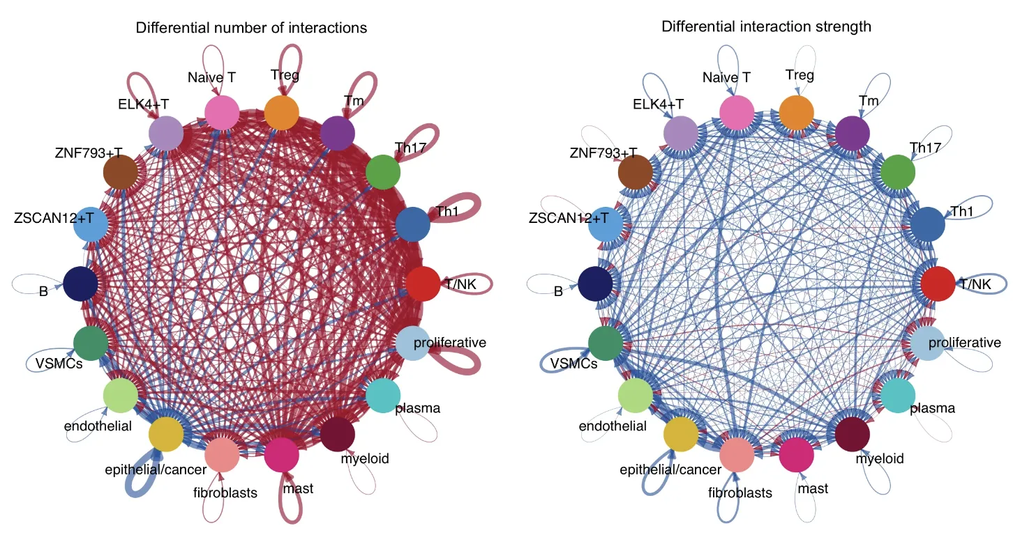
比较不同细胞群体之间的互作数量和强度

netVisual_diffInteraction(cellchat, weight.scale = T)
netVisual_diffInteraction(cellchat, weight.scale = T, measure = "weight")

通过圆形图可视化两个数据集中细胞间通讯网络中相互作用数量的差异或相互作用强度，其中红色或者蓝色的着色边代表与第一个数据集相比，第二个数据集中上调或者下调的信号。分组顺序是按照object.list中的顺序而定的。

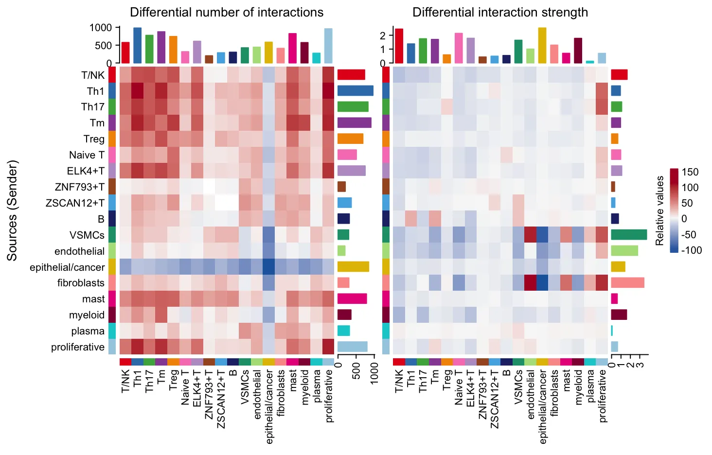
显示两个数据集中不同细胞群体间相互作用数量或相互作用强度的热图

gg1 <- netVisual_heatmap(cellchat)
#> Do heatmap based on a merged object
gg2 <- netVisual_heatmap(cellchat, measure = "weight")
#> Do heatmap based on a merged object
gg1 + gg2

weight.max <- getMaxWeight(object.list, attribute = c("idents","count"))
par(mfrow = c(1,2), xpd=TRUE)
for (i in 1:length(object.list)) {
  netVisual_circle(object.list[[i]]@net$count, weight.scale = T, label.edge= F, edge.weight.max = weight.max[2], edge.width.max = 12, title.name = paste0("Number of interactions - ", names(object.list)[i]))
}

顶部彩色条形图表示热图中显示的每列绝对值之和（传入信号）。右侧彩色条形图表示每行绝对值之和（传出信号）。因此，条形高度表示两个条件之间交互数量或交互强度变化的程度。在颜色条中，红色或者蓝色表示与第一个数据集相比，第二个数据集中上调或者下调的信号。感觉热图更直观，比如成纤维细胞和肿瘤细胞之间的交互呈现了右半结肠癌相对于左半结肠癌更少的互作数量，但是确有更显著的互作强度！

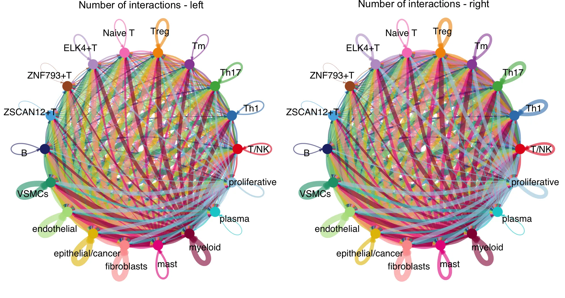
Circle图显示多个数据集中不同细胞群体之间的相互作用数量或相互作用强度

weight.max <- getMaxWeight(object.list, attribute = c("idents","count"))
par(mfrow = c(1,2), xpd=TRUE)
for (i in 1:length(object.list)) {
  netVisual_circle(object.list[[i]]@net$count, weight.scale = T, label.edge= F, edge.weight.max = weight.max[2], edge.width.max = 12, title.name = paste0("Number of interactions - ", names(object.list)[i]))
}

Circle图显示多个数据集中不同细胞群体之间的相互作用数量或相互作用强度

Circle图显示粗细胞类型之间的相互作用数量或相互作用强度差异

这里笔者瞎分一下，没有任何生物学意义哈，如果是自己的数据集，可以按照研究目的进行分组~

# 按照celltype_order进行分组
celltype_order
# 分组，这里笔者瞎分一下，没有任何生物学意义哈
group.cellType <- c(rep("T/NK", 9), rep("Group1", 4), rep("Group2", 5))
group.cellType <- factor(group.cellType, levels = c("T/NK", "Group1", "Group2"))
object.list <- lapply(object.list, function(x) {mergeInteractions(x, group.cellType)})
cellchat <- mergeCellChat(object.list, add.names = names(object.list))

weight.max <- getMaxWeight(object.list, slot.name = c("idents", "net", "net"), attribute = c("idents","count", "count.merged"))
# interactions
par(mfrow = c(1,2), xpd=TRUE)
for (i in 1:length(object.list)) {
  netVisual_circle(object.list[[i]]@net$count.merged, weight.scale = T, label.edge= T, edge.weight.max = weight.max[3], edge.width.max = 12, title.name = paste0("Number of interactions - ", names(object.list)[i]))
}

# weight.merged
par(mfrow = c(1,2), xpd=TRUE)
netVisual_diffInteraction(cellchat, weight.scale = T, measure = "count.merged", label.edge = T)
netVisual_diffInteraction(cellchat, weight.scale = T, measure = "weight.merged", label.edge = T)

不同组别之间的互作数量和强度

5.在二维空间中比较主要来源和目标

识别发送或接收信号发生显著变化的细胞群体

num.link <- sapply(object.list, function(x) {rowSums(x@net$count) + colSums(x@net$count)-diag(x@net$count)})
weight.MinMax <- c(min(num.link), max(num.link)) # control the dot size in the different datasets
gg <- list()
for (i in 1:length(object.list)) {
  gg[[i]] <- netAnalysis_signalingRole_scatter(object.list[[i]], title = names(object.list)[i], weight.MinMax = weight.MinMax)
}

patchwork::wrap_plots(plots = gg)

似乎差别不是那么明显。

官网示例数据，与NL相比，Inflam.DC 和 cDC1 成为 LS 中主要的来源和靶点之一。成纤维细胞群体也成为 LS 中的主要来源

识别特定细胞群体的信号变化

# 可视化从left样本到right样本的发出与接收信号差异变化
gg1 <- netAnalysis_signalingChanges_scatter(cellchat, idents.use = "Th1", signaling.exclude = "MIF")

gg2 <- netAnalysis_signalingChanges_scatter(cellchat, idents.use = "Treg", signaling.exclude = c("MIF"))

patchwork::wrap_plots(plots = list(gg1,gg2))

按照github中作者的解释，正值表示在第二种情况中升高，负值表示在第一种情况中升高。对应到我们这里也就是说左半结肠癌中的Th1细胞中CD99、MHC-1、COLLAGEN、CLEC升高，右半结肠中的Th1细胞中MHC-II、IL-2、CXCL升高。

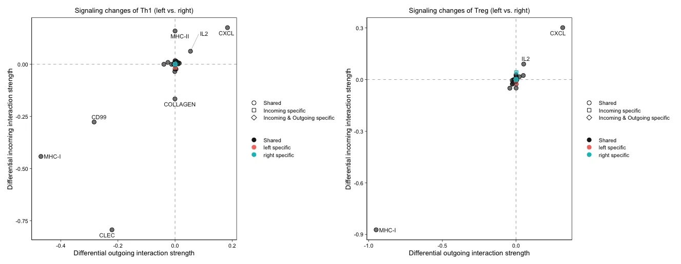
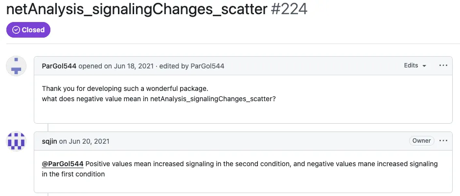
github回答：https://github.com/sqjin/CellChat/issues/224

6.识别具有不同相互作用强度的改变信号

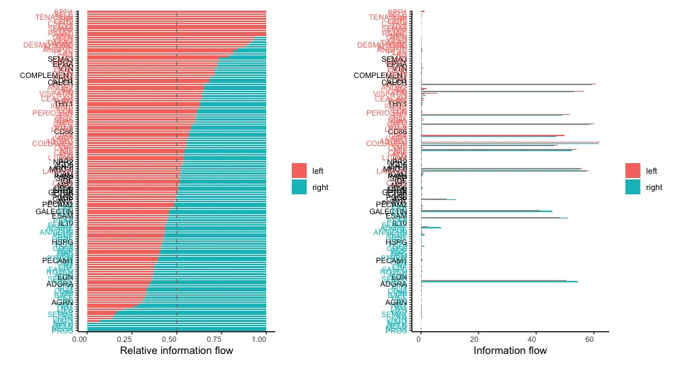
比较每个信号通路或配体-受体对的总体信息流。

gg1 <- rankNet(cellchat, mode = "comparison", measure = "weight", sources.use = NULL, targets.use = NULL, stacked = T, do.stat = TRUE)
gg2 <- rankNet(cellchat, mode = "comparison", measure = "weight", sources.use = NULL, targets.use = NULL, stacked = F, do.stat = TRUE)

gg1 + gg2

可以观察左右半结肠癌信号流的情况。

比较与每个细胞群体相关的传出和传入信号模式

library(ComplexHeatmap)
i = 1
# combining all the identified signaling pathways from different datasets 
pathway.union <- union(object.list[[i]]@netP$pathways, object.list[[i+1]]@netP$pathways)
ht1 = netAnalysis_signalingRole_heatmap(object.list[[i]], pattern = "outgoing", signaling = pathway.union, title = names(object.list)[i], width = 5, height = 6)
ht2 = netAnalysis_signalingRole_heatmap(object.list[[i+1]], pattern = "outgoing", signaling = pathway.union, title = names(object.list)[i+1], width = 5, height = 6)
draw(ht1 + ht2, ht_gap = unit(0.5, "cm"))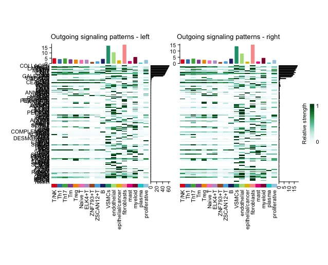

7.识别上调和下调的信号配体-受体对

通过比较通信概率来识别功能障碍的信号

netVisual_bubble(cellchat, sources.use = 4, targets.use = c(5:7),  comparison = c(1, 2), angle.x = 45)

gg1 <- netVisual_bubble(cellchat, sources.use = 4, targets.use = c(5:7),  comparison = c(1, 2), max.dataset = 2, title.name = "Increased signaling in Left", angle.x = 45, remove.isolate = T)
#> Comparing communications on a merged object
gg2 <- netVisual_bubble(cellchat, sources.use = 4, targets.use = c(5:7),  comparison = c(1, 2), max.dataset = 1, title.name = "Decreased signaling in right", angle.x = 45, remove.isolate = T)
#> Comparing communications on a merged object
gg1 + gg2

CellChat 可以比较来自特定细胞群体的 L-R 对介导的通信概率与其他细胞群体之间的通信概率。

通过差异表达分析识别功能障碍性信号

对每个细胞群体在两种生物条件之间进行差异表达分析，然后根据sender细胞中配体的倍数变化和接收细胞中受体的倍数变化来获得上调和下调的信号。

# 设定"实验组"
pos.dataset = "right"
features.name = paste0(pos.dataset, ".merged")
cellchat <- identifyOverExpressedGenes(cellchat, group.dataset = "datasets", pos.dataset = pos.dataset, features.name = features.name, only.pos = FALSE, thresh.pc = 0.1, thresh.fc = 0.05,thresh.p = 0.05, group.DE.combined = FALSE) 

net <- netMappingDEG(cellchat, features.name = features.name, variable.all = TRUE)
net.up <- subsetCommunication(cellchat, net = net, datasets = "left",ligand.logFC = 0.05, receptor.logFC = NULL)
net.down <- subsetCommunication(cellchat, net = net, datasets = "right",ligand.logFC = -0.05, receptor.logFC = NULL)

gene.up <- extractGeneSubsetFromPair(net.up, cellchat)
gene.down <- extractGeneSubsetFromPair(net.down, cellchat)

# 自定义特征和感兴趣的细胞群体找到所有显著的outgoing/incoming/both向信号
df <- findEnrichedSignaling(object.list[[2]], features = c("CCL19", "CXCL12"), idents = c("Treg", "Tm"), pattern ="outgoing")

net.up

可视化已识别的上调/下调信号配体-受体对

# 气泡图
pairLR.use.up = net.up[, "interaction_name", drop = F]
gg1 <- netVisual_bubble(cellchat, pairLR.use = pairLR.use.up, sources.use = 4, targets.use = c(5:11), comparison = c(1, 2),  angle.x = 90, remove.isolate = T,title.name = paste0("Up-regulated signaling in ", names(object.list)[2]))
pairLR.use.down = net.down[, "interaction_name", drop = F]
gg2 <- netVisual_bubble(cellchat, pairLR.use = pairLR.use.down, sources.use = 4, targets.use = c(5:11), comparison = c(1, 2),  angle.x = 90, remove.isolate = T,title.name = paste0("Down-regulated signaling in ", names(object.list)[2]))
gg1 + gg2

# 和弦图
# Chord diagram
par(mfrow = c(1,2), xpd=TRUE)
netVisual_chord_gene(object.list[[2]], sources.use = 4, targets.use = c(5:11), slot.name = 'net', net = net.up, lab.cex = 0.8, small.gap = 3.5, title.name = paste0("Up-regulated signaling in ", names(object.list)[2]))
netVisual_chord_gene(object.list[[1]], sources.use = 4, targets.use = c(5:11), slot.name = 'net', net = net.down, lab.cex = 0.8, small.gap = 3.5, title.name = paste0("Down-regulated signaling in ", names(object.list)[2]))

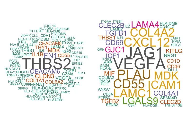
# 词云图
library(wordcloud)
computeEnrichmentScore(net.down, species = 'human', variable.both = TRUE)
computeEnrichmentScore(net.up, species = 'human', variable.both = TRUE)

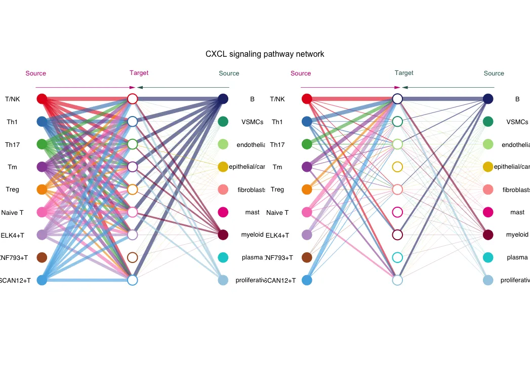
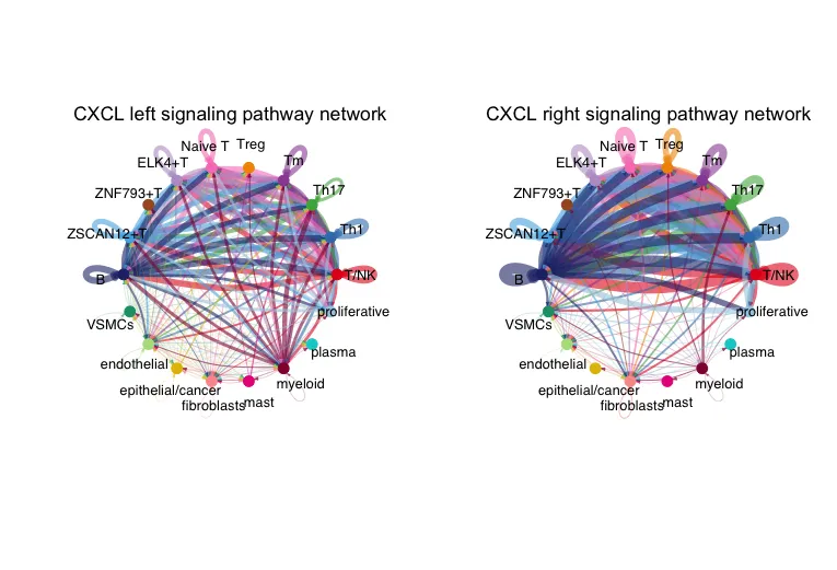
可视化，使用层次图、圆形图或弦图直观比较细胞间通讯

pathways.show <- c("CXCL") 
weight.max <- getMaxWeight(object.list, slot.name = c("netP"), attribute = pathways.show) # control the edge weights across different datasets
par(mfrow = c(1,2), xpd=TRUE)
for (i in 1:length(object.list)) {
  netVisual_aggregate(object.list[[i]], signaling = pathways.show, layout = "circle", edge.weight.max = weight.max[1], edge.width.max = 10, signaling.name = paste(pathways.show, names(object.list)[i]))
}

pathways.show <- c("CXCL") 
par(mfrow = c(1,2), xpd=TRUE)
ht <- list()
for (i in 1:length(object.list)) {
  ht[[i]] <- netVisual_heatmap(object.list[[i]], signaling = pathways.show, color.heatmap = "Reds",title.name = paste(pathways.show, "signaling ",names(object.list)[i]))
}
#> Do heatmap based on a single object 
#> 
#> Do heatmap based on a single object
ComplexHeatmap::draw(ht[[1]] + ht[[2]], ht_gap = unit(0.5, "cm"))

# Chord diagram
pathways.show <- c("CXCL") 
par(mfrow = c(1,2), xpd=TRUE)
for (i in 1:length(object.list)) {
  netVisual_aggregate(object.list[[i]], signaling = pathways.show, layout = "chord", signaling.name = paste(pathways.show, names(object.list)[i]))
}
# Chord diagram 的另外一种形式
# group.cellType <- c(rep("FIB", 4), rep("DC", 4), rep("TC", 4)) # grouping cell clusters into fibroblast, DC and TC cells
# names(group.cellType) <- levels(object.list[[1]]@idents)
# pathways.show <- c("CXCL") 
# par(mfrow = c(1,2), xpd=TRUE)
# for (i in 1:length(object.list)) {
#   netVisual_chord_cell(object.list[[i]], signaling = pathways.show, group = group.cellType, title.name = paste0(pathways.show, " signaling network - ", names(object.list)[i]))
# }

par(mfrow = c(1, 2), xpd=TRUE)
for (i in 1:length(object.list)) {
  netVisual_chord_gene(object.list[[i]], sources.use = 4, targets.use = c(5:6), lab.cex = 0.5, title.name = paste0("Signaling from Tm - ", names(object.list)[i]))
}

# compare all the interactions sending from fibroblast to inflamatory immune cells
# par(mfrow = c(1, 2), xpd=TRUE)
# for (i in 1:length(object.list)) {
#   netVisual_chord_gene(object.list[[i]], sources.use = c(1,2, 3, 4), targets.use = c(8,10),  title.name = paste0("Signaling received by Inflam.DC and .TC - ", names(object.list)[i]), legend.pos.x = 10)
# }

可视化结果，可以自行尝试。

可视化，表达情况

cellchat@meta$datasets = factor(cellchat@meta$datasets, levels = c("left", "right")) # set factor level
plotGeneExpression(cellchat, signaling = "CXCL", split.by = "datasets", colors.ggplot = T, type = "violin")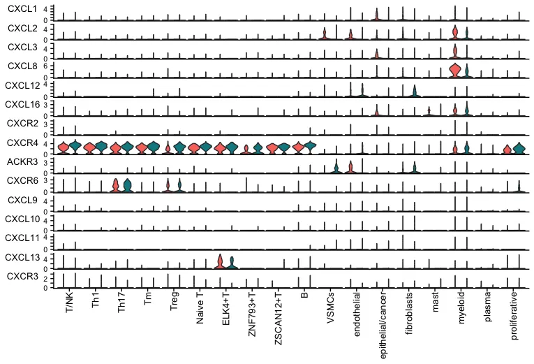

参考资料：

Inference and analysis of cell-cell communication using CellChat. Nat Commun. 2021 Feb 17;12(1):1088.
CellChat for systematic analysis of cell-cell communication from single-cell transcriptomics. Nat Protoc. 2025 Jan;20(1):180-219.
Cellchat github：https://github.com/jinworks/CellChat
CellChatDB更新：https://htmlpreview.github.io/?https://github.com/jinworks/CellChat/blob/master/tutorial/Update-CellChatDB.html
生信技能树：https://mp.weixin.qq.com/s/9Q4rxGKFo_jD8vBkuOzTbQ
生信方舟：https://mp.weixin.qq.com/s/yEXqbo6pBNuIq_tMSsrZig

致谢：感谢曾老师以及生信技能树团队全体成员。更多精彩内容可关注公众号：生信技能树，单细胞天地，生信菜鸟团等公众号。

注：若对内容有疑惑或者有发现明确错误的朋友，请联系后台(欢迎交流)。更多相关内容可关注公众号：生信方舟

- END -

原创声明：本文系作者授权腾讯云开发者社区发表，未经许可，不得转载。

如有侵权，请联系 cloudcommunity@tencent.com 删除。

数据挖掘

原创声明：本文系作者授权腾讯云开发者社区发表，未经许可，不得转载。

如有侵权，请联系 cloudcommunity@tencent.com 删除。

数据挖掘

#单细胞