
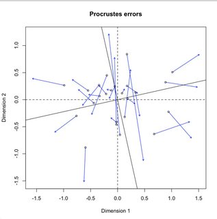
如何用Python (SciPy、NumPy和Matplotlib)绘制R的素食者::Pro壳?
我正在学习普罗甲壳动物分析的纯素教程:
https://www.rdocumentation.org/packages/vegan/versions/2.4-2/topics/procrustes
# Load data
library(vegan)
data(varespec)

# Ordinations
vare.dist <- vegdist(wisconsin(varespec))
mds.null <- monoMDS(vare.dist, y = cmdscale(vare.dist))
mds.alt <- monoMDS(vare.dist)

# Run procrustes
vare.proc <- procrustes(mds.alt, mds.null)

# Summary of procrustes
summary(vare.proc)
Call:
procrustes(X = mds.alt, Y = mds.null)

Number of objects: 24    Number of dimensions: 2

Procrustes sum of squares:
 13.99951
Procrustes root mean squared error:
 0.7637492
Quantiles of Procrustes errors:
       Min         1Q     Median         3Q        Max
0.08408327 0.23038165 0.49316643 0.65854198 1.99105837

Rotation matrix:
          [,1]       [,2]
[1,] 0.9761893  0.2169202
[2,] 0.2169202 -0.9761893

 of averages:
              [,1]          [,2]
[1,] -2.677059e-17 -5.251452e-18

Scaling of target:
[1] 0.6455131

plot(vare.proc)
现在,使用Python,我可以选择:
# Returns
mtx1: array_like
A standardized version of data1.

mtx2: array_like
The orientation of data2 that best fits data1. Centered, but not necessarily .

disparity: float
as defined above.R(N, N): ndarray
The matrix solution of the orthogonal Procrustes problem. Minimizes the Frobenius norm of (A @ R) - B, subject to R.T @ R = I.
scale: float
Sum of the singular values of A.T @ B.我的问题:
- 哪种实现更类似于
vegan::procrustes、scipy.spatial.procrustes或scipy.linalg.orthogonal_procrustes - 如何使用输出来生成上面的图(在Matplotlib中,不是通过Rpy2)?
编辑:
使用@凯特对密谋的回答和我的补充答案来实现SciPy/NumPy,应该能够准确地使用来自PyData的标准包来再现PyData中的纯素分析。
编辑2:
为了防止它对任何人有帮助,我在我的Procrustes python包中实现了vegan和Protest (以及这里描述的绘图方法):https://github.com/jolespin/soothsayer/blob/60accb669062c559ba785be201deddeede26a049/soothsayer/ordination/ordination.py#L715
回答 4
Stack Overflow用户
发布于 2022-01-28 18:40:34
vegan包在monoMDS中运行的方式似乎与Python使用的任何方法不一致。vegan中的代码都是基于Fortran的。您可以将Fortan链接到Python,就像在R中一样。
当缩放不同时,vare.proc内部的旋转矩阵与旋转矩阵(数组?)完全相同。在vare_proc上面的Python编码对象中。我觉得这很有趣。
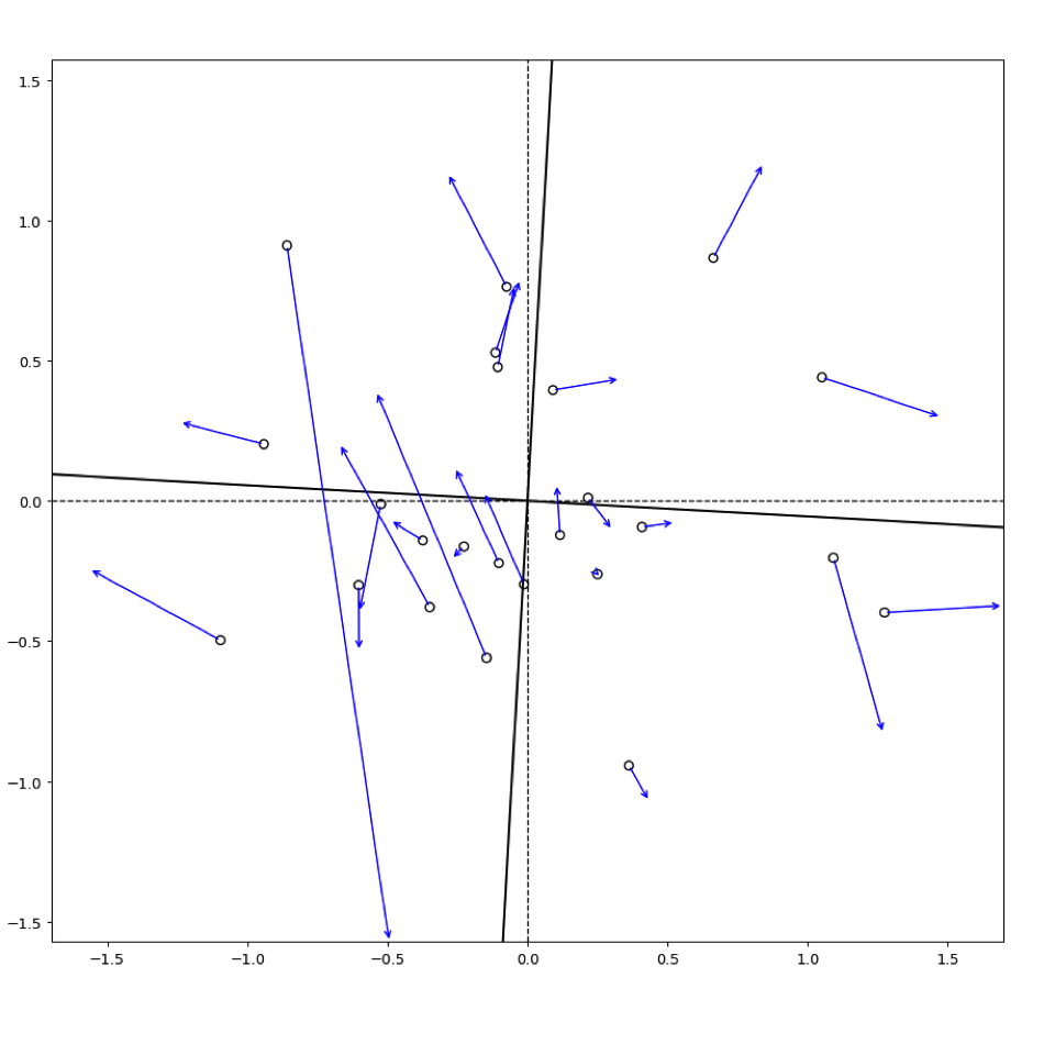
如果我为您的对象vare.proc引入R中的内容片段,我可以做出精确的图形。
首先,我使用在Python和R之间共享对象。
# compare to R
# vpR = vareProc$rotation
vpR_py = r.vpR
# vpYrot = vareProc$Yrot
vpYrot_py = r.vpYrot
# vpX = vareProc$X
vpX_py = r.vpX
然后我用这些对象来复制
# build the plot exactly like vegan
# using https://github.com/vegandevs/vegan/blob/master/R/plot.procrustes.R
tails = vpYrot_py
heads = vpX_py

# find the ranges
xMax = max(abs(np.hstack((tails[:,0], heads[:,0]))))
yMax = max(abs(np.hstack((tails[:,1], heads[:,1]))))

plt.figure(dpi = 100)
fig, ax = plt.subplots()
ax.set_aspect('equal')
ax.set_xlim(-xMax, xMax)
ax.set_ylim(-yMax, yMax)

# add points
ax.scatter(x = tails[:,0],
           y = tails[:,1],
           facecolors = 'none',
           edgecolors = 'k')

# add origin axes
ax.axhline(y = 0, color='k', ls = '--', linewidth = 1) # using dashed for origin
ax.axvline(x = 0, color='k', ls = '--', linewidth = 1)

# add rotation axes
ax.axline(xy1 = (0, 0), color = 'k',
          slope = vpR_py[0, 1]/vpR_py[0, 0])
ax.axline(xy1 = (0, 0), color = 'k',
          slope = vpR_py[1, 1]/vpR_py[1, 0])

# add arrows
for i in range(0, len(tails)):
  ax.annotate("", xy = heads[i,:],
              xycoords = 'data',
              xytext = tails[i,:],
              arrowprops=dict(arrowstyle="->",
                              color = 'blue'))

plt.tight_layout(pad = 2)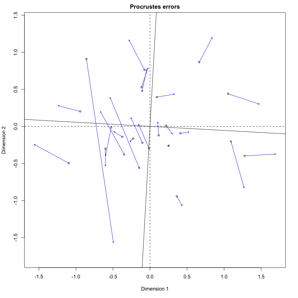
plt.show()来自matplotlib
来自vegan
Stack Overflow用户
发布于 2022-01-27 03:09:47
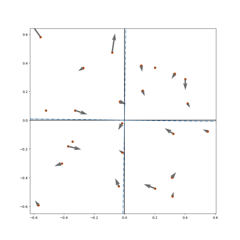
不完全一样,但我觉得很接近。
为此,我将varespec数据引入Python。然后尝试模仿vegan包(和您的代码)所采取的操作。沿着这些思路,我坚持您使用的对象名称(在大多数情况下)。
必须有更简单的方法来做到这一点。
import scipy.spatial.distance as ssd
import sklearn.manifold as sm #  MDS, smacof
import procrustes
import numpy as np
import matplotlib.pyplot as plt
import pandas as pd

wVares_py = r.wVares # I brought in the varespec data from R (named wVares)
# find the distance
vare_dist = ssd.pdist(wVares_py, 'braycurtis')
# make it square (Required for MDS and smaof
vare_dist = ssd.squareform(vare_dist)

mds = sm.MDS(metric = False, dissimilarity = 'precomputed')
mds_alt = mds.fit_transform(vare_dist)
mds_null = sm.smacof(vare_dist, metric = False, init = mds_alt)

vare_proc = procrustes.rotational(mds_alt, mds_null[0], translate = False)

# create an array that represents the axes at the origin, then rotate them
xAx = np.array([[-.4, 0],[.4, 0]])
yAx = np.array([[0, .4], [0, -.4]])

# create the rotated origins
xHat = vare_proc["t"] * xAx
yHat = vare_proc["t"] * yAx

# add line segments
vareA = pd.DataFrame(vare_proc.new_a, columns = ['x1', 'y1'])
vareB = pd.DataFrame(vare_proc.new_b, columns = ['x2', 'y2'])
df = pd.concat([vareA, vareB], axis = 1)

# now find the differences
df['dx'] = df.x2 - df.x1
df['dy'] = df.y2 - df.y1
现在一切都准备好了。
plt.figure(figsize = (10, 10), dpi = 100)
fig, ax = plt.subplots()
# plot the points
# plot the points
ax.scatter(vare_proc.new_a[:, 0],
           vare_proc.new_a[:, 1],
           marker = 'o',
           label = 'a',
           c = '#cc5500')
# plot the x, y axes
ax.axhline(y=0, color='k')
ax.axvline(x=0, color='k')
# plot the rotated origin
ax.axline(xHat[:,0], xHat[:,1], linestyle = '-.')
ax.axline(yHat[:,0], yHat[:,1], linestyle = '-.')
# add arrows to show the direction per point
ax.quiver(df.x1, df.y1, df.dx, df.dy, units='xy', color = 'gray', scale=.7)
plt.show()
Stack Overflow用户
发布于 2022-02-02 20:33:35
下面是如何仅使用vegan和NumPy在SciPy中再现SciPy分析。关于如何情节的上下文,请参阅上面的@Kat答案:
# Get X and Y which are the first 2 embeddings
# -------------------------------------------
# X <- scores(X, display = scores, ...)
mds_null = pd.read_csv("https://pastebin.com/raw/c1Zwb4pu", index_col=0, sep="\t")
X_original = mds_null.values
# X_original[:5]
# array([[-0.28600328, -0.23135498],
#        [ 0.00510282, -0.39170001],
#        [ 0.80888622,  1.18656269],
#        [ 1.44897916, -0.18887702],
#        [ 0.54496396, -0.09403705]])

# Y <- scores(X, display = scores, ...)
mds_alt = pd.read_csv("https://pastebin.com/raw/UMGLgXmu", index_col=0, sep="\t")
Y_original = mds_alt.values
# Y_original[:5]
# array([[ 0.2651293 ,  0.09755548],
#        [ 0.17639036,  0.45328207],
#        [-0.16167398, -1.42304932],
#        [-1.44706047,  0.3966337 ],
#        [-0.49825949,  0.15239689]])


# Procrustes in VEGAN
# ----------------
procrustes_result = vegan.procrustes(X_original, Y_original, scale=True, symmetric=False, scores="sites")

# Rotation matrix from VEGAN
A = np.array(dict(procrustes_result.items())["rotation"])
# A
# # array([[-0.98171787, -0.19034186],
# #        [ 0.19034186, -0.98171787]])

# Center the X and Y data
# -----------------------
X_mean = X_original.mean(axis=0)
X = X_original - X_mean
Y_mean = Y_original.mean(axis=0)
Y = Y_original - Y_mean

# # Rotation matrix from SciPy
# ----------------------------
A, sca = orthogonal_procrustes(X,Y)
# A
# array([[-0.98171787,  0.19034186],
#        [-0.19034186, -0.98171787]])


# Manual calculation
# ------------------
# np.linalg.svd returns:
# u{ (…, M, M), (…, M, K) } array
# Unitary array(s). The first a.ndim - 2 dimensions have the same size as those of the input a. The size of the last two dimensions depends on the value of full_matrices. Only returned when compute_uv is True.

# s(…, K) array
# Vector(s) with the singular values, within each vector sorted in descending order. The first a.ndim - 2 dimensions have the same size as those of the input a.

# vh{ (…, N, N), (…, K, N) } array
# Unitary array(s). The first a.ndim - 2 dimensions have the same size as those of the input a. The size of the last two dimensions depends on the value of full_matrices. Only returned when compute_uv is True.

XY = np.dot(X.T, Y) # crossprod(X,Y)
U,s,Vh = np.linalg.svd(XY)
V = Vh.T
A = np.dot(V, U.T)
# A
# array([[-0.98171787, -0.19034186],
#        [ 0.19034186, -0.98171787]])

# Reproduce the Yrot object
# -------------------------
scale = True
symmetric = False

# Yrot from VEGAN
Yrot = np.array(dict(procrustes_result.items())["Yrot"])
# Yrot[:5]
# array([[-0.20919556, -0.12656386],
#        [-0.07519809, -0.41418755],
#        [-0.09706039,  1.23572329],
#        [ 1.29483042, -0.098617  ],
#        [ 0.44844991, -0.04740275]])

# NumPy implementation
# ctrace <- function(MAT) sum(MAT^2)
def ctrace(MAT):
    return np.sum(MAT**2)

# if (scale) {
#     c <- sum(sol$d)/ctrace(Y)
if scale:
    c = np.sum(s)/ctrace(Y)

# Yrot <- c * Y %*% A
Yrot = c * np.dot(Y,A)
Yrot[:5]
# array([[-0.20919556, -0.12656386],
#        [-0.07519809, -0.41418755],
#        [-0.09706039,  1.23572329],
#        [ 1.29483042, -0.098617  ],
# [ 0.44844991, -0.04740275]])https://stackoverflow.com/questions/70870829
复制相似问题
腾讯云开发者
