
如何巧妙地启用二级y轴&获得更好的视觉效果
如何巧妙地启用二级y轴&获得更好的视觉效果
提问于 2020-09-26 07:05:04
我正在创建OHLC图形,使用与和添加线条图到相同的绘图,以显示移动平均值& RSI,可以启用或禁用点击图例。
我正在使用下面的教程在下面的链接中提供代码创建所需的图表
#https://chart-studio.plotly.com/~jackp/17421/plotly-candlestick-chart-in-python/#/

import time


Mstart = time.process_time()

import plotly.graph_objects as go
from plotly.subplots import make_subplots
import plotly.io as pio


from plotly.offline import iplot
# Calling Numpy package to manipulate numbers
import numpy as np

# Calling Pandas to create dataframe
import pandas as pd

#importing ta-lib to calculate Technical indicators
import talib as ta

import datetime
from datetime import date as dt


# ----------------------- Loading data from csv file --------------------------------

VipData = pd.read_csv(r"C:\xxxxxxxx\data.csv")


#  ---------------------------   Generating Technical indicator features --------------------------
VipData['RSI7']= ta.RSI(VipData['Close'].values, timeperiod=7)

def bbp(price):
    #print(price)
    up, mid, low = ta.BBANDS(price, timeperiod=20, nbdevup=2, nbdevdn=2, matype=0)
    bbp = (VipData['Close'] - low) / (up - low)
    return up, mid, low, bbp

VipData['BB_up'],VipData['BB_mid'],VipData['BB_low'],VipData['BBP']=bbp(VipData.Close)
VipData['AD']=ta.AD(VipData.High, VipData.Low, VipData.Close, VipData.Volume)
VipData['OBV'] = ta.OBV(VipData.Close, VipData.Volume)
VipData['EMA12']=ta.EMA(VipData.Close, timeperiod=12)
VipData['EMA26']=ta.EMA(VipData.Close, timeperiod=26)
VipData['MA10'] = ta.MA(VipData.Close, timeperiod=10, matype=0)
VipData['MA50'] = ta.MA(VipData.Close, timeperiod=50, matype=0)
VipData['MP'] = ta.MIDPOINT(VipData.Close, timeperiod=14)
VipData['SMA10']= ta.SMA(VipData.Close, timeperiod=10)
VipData['SMA42']= ta.SMA(VipData.Close, timeperiod=42)
VipData['ADX'] = ta.ADX(VipData.High, VipData.Low, VipData.Close, timeperiod=14)
VipData['CCI'] = ta.CCI(VipData.High, VipData.Low, VipData.Close, timeperiod=14)

def macd(close):
    macd, macdsignal, macdhist = ta.MACD(close, fastperiod=12, slowperiod=26, signalperiod=9)
    return macd, macdsignal, macdhist

VipData['MACD'],VipData['MACDSig'],VipData['MACDHist'] = macd(VipData.Close)
VipData['MDI'] = ta.MINUS_DI(VipData.High, VipData.Low, VipData.Close, timeperiod=14)
VipData['PDM'] = ta.PLUS_DM(VipData.High, VipData.Low, timeperiod=14)
VipData['ATR'] = ta.ATR(VipData.High, VipData.Low, VipData.Close, timeperiod=14)

#--------------------------- Creating Chart ------------------------------------------------------
Cstart = time.process_time()
fig = make_subplots(specs=[[{"secondary_y": True}]])

INCREASING_COLOR = '#90ee90'
DECREASING_COLOR = '#ff0000'

#Create the layout object
annotations = []
annotations.append(go.layout.Annotation(x= VipData['Datetime'].iloc[VipData['Close'].idxmin()],
                                        y=VipData['Close'].iloc[VipData['Close'].idxmin()],
                                        showarrow=True,
                                        arrowhead=1,
                                        arrowcolor="purple",
                                        arrowsize=2,
                                        arrowwidth=2,
                                        text="Low"))

annotations.append(go.layout.Annotation(x= VipData['Datetime'].iloc[VipData['Close'].idxmax()],
                                        y=VipData['Close'].iloc[VipData['Close'].idxmax()],
                                        showarrow=True,
                                        arrowhead=1,
                                        arrowcolor="purple",
                                        arrowsize=2,
                                        arrowwidth=2,
                                        text="High"))

layout = dict(
        title="VIP Chart",
        xaxis=go.layout.XAxis(title=go.layout.xaxis.Title( text="Time (IST)"), rangeslider=dict (visible = True)),
        yaxis=go.layout.YAxis(title=go.layout.yaxis.Title( text="Price - Indian Rupees"),domain = [0, 0.2]),
        yaxis2 = go.layout.YAxis(domain = [0.2, 0.8],title=go.layout.yaxis.Title( text="Indicator Values")),
        legend = dict(orientation = 'h', y=0.9, x=0.3, yanchor='bottom'),
        margin = dict( t=29, b=20, r=20, l=20 ),
        width=800,
        height=600,
        annotations=annotations
)

#Creating OHLC Chart
data = [ dict(
    type = 'ohlc',
    open = VipData.Open,
    high = VipData.High,
    low = VipData.Low,
    close = VipData.Close,
    x = VipData.Datetime,
    yaxis = 'y2',
    name = 'OHLC',
    increasing = dict( line = dict( color = INCREASING_COLOR ) ),
    decreasing = dict( line = dict( color = DECREASING_COLOR ) ),
) ]

layout=dict()

fig = dict( data=data, layout=layout )

#Adding moving average
fig['data'].append( dict( x=list(VipData.Datetime), y=list(VipData.MA10), type='scatter', mode='lines',
                         line = dict( width = 1 ),
                         marker = dict( color = '#E377C2' ),
                         yaxis = 'y2', name='Moving Average' ) )

#Add RSI chart
fig['data'].append( dict( x=VipData.Datetime, y=VipData.RSI7,
                         marker=dict( color='#000' ),
                         type='scatter', yaxis='y', secondary_y=True, name='RSI' ) )

#Add volume bollinger bands
fig['data'].append( dict( x=VipData.Datetime, y=VipData.BB_up, type='scatter', yaxis='y2',
                         line = dict( width = 1 ),
                         marker=dict(color='#b41c1c'), hoverinfo='none',
                         legendgroup='Bollinger Bands', name='Bollinger Bands'))

fig['data'].append( dict( x=VipData.Datetime, y=VipData.BB_low, type='scatter', yaxis='y2',
                         line = dict( width = 1 ),
                         marker=dict(color='#b41c1c'), hoverinfo='none',
                         legendgroup='Bollinger Bands', showlegend=False ))

CRstart = time.process_time()

pio.renderers.default = "browser"

iplot( fig, filename = 'candlestick-test-3', validate = False )
#iplot( fig, validate = False )

Cend = time.process_time()

CRtime = Cend - CRstart
CTime = Cend-Cstart

print(f'Chart rendered in {CRtime} secs')
print(f'Chart created in {CTime} secs')
图表正在创建,但我遇到了两个问题:
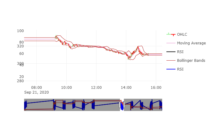
- 两个Y轴的值都在相同的边,图的左边是如何在右边显示第二个y轴的。添加图片供您参考。
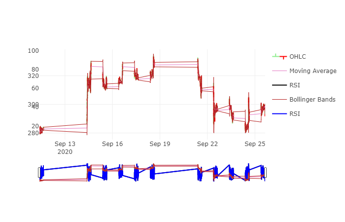
- 因为这是一个日内数据,每隔1分钟就会很密集,所以当我放大到同样的数据时,烛台变得非常小。如何增大大小相同。我知道OHLC是非常接近彼此,但我仍然希望有更大的烛台,以更好的能见度。我怎么才能做同样的事。图片供您参考
谢谢你的时间和努力帮助我。
问候苏迪尔
回答 1
Stack Overflow用户
回答已采纳
发布于 2020-09-26 12:08:31
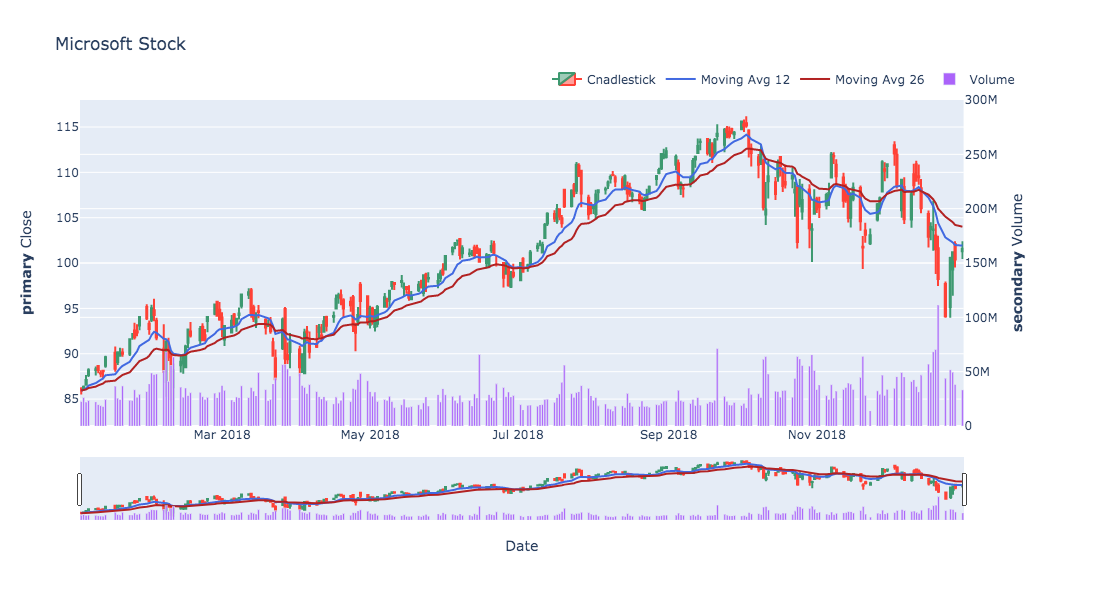
这是一个有趣的问题,所以我添加了第二个y轴设置和移动平均值,指的是官方的参考文献。限制滑块的周期也会扩大烛台;我没有看到任何设置可以使烛台上的盒子变大。
import plotly.graph_objects as go
import numpy as np
import pandas as pd
import pandas_datareader.data as web
import datetime
from plotly.subplots import make_subplots


start = datetime.datetime(2018, 1, 1)
end = datetime.datetime(2019, 1, 1)
df = web.DataReader("MSFT", 'yahoo', start, end)
df.reset_index(inplace=True)
# moving average
exp12 = df['Close'].ewm(span=12, adjust=False).mean()
exp26 = df['Close'].ewm(span=26, adjust=False).mean()
macd = exp12 - exp26
signal = macd.ewm(span=9, adjust=False).mean()

# Create figure with secondary y-axis
fig = make_subplots(specs=[[{"secondary_y": True}]])

fig.add_trace(go.Candlestick(x=df['Date'], open=df['Open'], high=df['High'], low=df['Low'], close=df['Close'],
                             yaxis='y1', name='Cnadlestick'))

fig.add_trace(go.Scatter(x=df['Date'], y=exp12, name='Moving Avg 12',
                        line=dict(color='royalblue',width=2)))

fig.add_trace(go.Scatter(x=df['Date'], y=exp26, name='Moving Avg 26',
                        line=dict(color='firebrick',width=2)))

fig.add_trace(go.Bar(x=df['Date'], y=df['Volume'], yaxis='y2', name='Volume'))

# Add figure title
fig.update_layout(
    width=1100,
    height=600,
    title_text="Microsoft Stock",
    yaxis_tickformat='M'
)

fig.update_layout(legend=dict(
    orientation="h",
    yanchor="bottom",
    y=1.02,
    xanchor="right",
    x=1
))

# Set x-axis title
fig.update_xaxes(title_text="Date")

# Set y-axes titles
fig.update_yaxes(title_text="<b>primary</b> Close", secondary_y=False)
fig.update_yaxes(title_text="<b>secondary</b> Volume", range=[0, 300000000], secondary_y=True)

fig.show()
页面原文内容由Stack Overflow提供。腾讯云小微IT领域专用引擎提供翻译支持
原文链接:
https://stackoverflow.com/questions/64074854
复制相关文章
相似问题
腾讯云开发者
