
logistic回归中决策边界的绘制
我正在一个小型数据集上运行逻辑回归,如下所示:

在实现梯度下降和成本函数之后,我在预测阶段获得了89%的精度,但是我想确定一切都是有序的,所以我试图绘制将两个数据集分开的决策分界线。
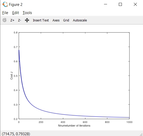
下面我给出了显示成本函数和θ参数的图表。可以看到,目前我打印的决定边界线不正确。
当我放大决策边界图时,我可以看到以下内容:
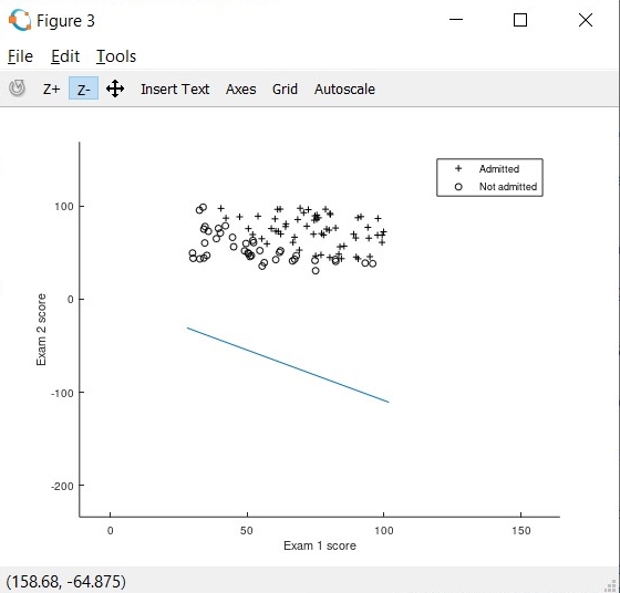
我的决策边界正在数据集下面绘制。需要注意的一点是,我使用了功能缩放。
下面是我使用的代码:
主程序
%% Initialization
clear ; close all; clc

%% Load Data
%  The first two columns contains the exam scores and the third column
%  contains the label.

data = load('ex2data1.txt');
X = data(:, [1, 2]); y = data(:, 3);

%% ==================== Part 1: Plotting ====================
%  We start the exercise by first plotting the data to understand the
%  the problem we are working with.

fprintf(['Plotting data with + indicating (y = 1) examples and o ' ...
         'indicating (y = 0) examples.\n']);

plotData(X, y);

% Put some labels
hold on;
% Labels and Legend
xlabel('Exam 1 score')
ylabel('Exam 2 score')

% Specified in plot order
legend('Admitted', 'Not admitted')
hold off;

fprintf('\nProgram paused. Press enter to continue.\n');
pause;


%% ============ Part 2: Compute Cost and Gradient ============
%  In this part of the exercise, you will implement the cost and gradient
%  for logistic regression. You neeed to complete the code in
%  costFunction.m

%  Setup the data matrix appropriately, and add ones for the intercept term
[m, n] = size(X);

%Normalize Feature
[X_norm mu sigma] = featureNormalize(X);

% Add intercept term to x and X_test
X = [ones(m, 1) X];
X_norm = [ones(m, 1) X_norm];

% Initialize fitting parameters
initial_theta = zeros(n + 1, 1);

% Compute and display initial cost and gradient
J = computeCostgrad(X_norm, y, initial_theta);

fprintf('Cost at initial theta (zeros): %f\n', J);
fprintf('Expected cost (approx): 0.693\n');


fprintf('\nProgram paused. Press enter to continue.\n');
pause;

%% ============= Part 2a: Gradient Descent =====================
alpha=0.1;
iter=1000;
[theta, J_hist]=gradientDescent(initial_theta, X_norm, y, alpha, iter);
fprintf('Theta found by gradient descent:\n');
fprintf('%f\n', theta);

% Plot the convergence graph
figure;
plot(1:numel(J_hist), J_hist, '-b', 'LineWidth', 2);
xlabel('Nnumelumber of iterations');
ylabel('Cost J');


% Plot Boundary
plotDecisionBoundary(theta, X, y);

% Put some labels
hold on;
% Labels and Legend
xlabel('Exam 1 score')
ylabel('Exam 2 score')

% Specified in plot order
legend('Admitted', 'Not admitted')
hold off;

fprintf('\nProgram paused. Press enter to continue.\n');
pause;

%% ============== Part 4: Predict and Accuracies ==============
%  After learning the parameters, you'll like to use it to predict the outcomes
%  on unseen data. In this part, you will use the logistic regression model
%  to predict the probability that a student with score 45 on exam 1 and
%  score 85 on exam 2 will be admitted.
%
%  Furthermore, you will compute the training and test set accuracies of
%  our model.
%
%  Your task is to complete the code in predict.m

%  Predict probability for a student with score 45 on exam 1
%  and score 85 on exam 2

%prob = sigmoid([1 45 85] * theta);
pred_admit=[45 85];
norm_pred_admit=[1,(pred_admit-mu)./sigma];
prob = norm_pred_admit*theta;
fprintf(['For a student with scores 45 and 85, we predict an admission ' ...
         'probability of %f\n'], prob);
fprintf('Expected value: 0.775 +/- 0.002\n\n');

% Compute accuracy on our training set
p = predict(theta, X_norm);

fprintf('Train Accuracy: %f\n', mean(double(p == y)) * 100);
fprintf('Expected accuracy (approx): 89.0\n');
fprintf('\n');
computeCostgrad
function [J] = computeCostgrad(X, y, theta)
  % Initialize some useful values
m = length(y); % number of training examples

% You need to return the following variables correctly
J = 0;


prediction=sigmoid(X*theta);
prob1=-y'*log(prediction);
prob0=(1-y')*log(1-prediction);
J=1/m*(prob1-prob0);
endfunction
gradientDescent
function [theta, J_hist] = gradientDescent(theta, X, y, alpha, iter)

   m=length(y);
   J_hist=zeros(iter, 1);
  for (i=1:iter)
  prediction=sigmoid(X*theta);
  err=prediction-y;
  newDecrement = (alpha * (1/m) * err' * X);
  theta=theta-newDecrement';
  J_hist(i)=computeCostgrad(X,y,theta);
  end

endfunction
plotDecisionBoundary
function plotDecisionBoundary(theta, X, y)
plotData(X(:,2:3), y);
hold on

if size(X, 2) <= 3
    % Only need 2 points to define a line, so choose two endpoints
    plot_x = [min(X(:,2))-2,  max(X(:,2))+2];

    % Calculate the decision boundary line
    plot_y = (-1./theta(3)).*(theta(2).*plot_x + theta(1));

    % Plot, and adjust axes for better viewing
    plot(plot_x, plot_y)

    % Legend, specific for the exercise
    legend('Admitted', 'Not admitted', 'Decision Boundary')
    axis([30, 100, 30, 100])
else
    % Here is the grid range
    u = linspace(-1, 1.5, 50);
    v = linspace(-1, 1.5, 50);

    z = zeros(length(u), length(v));
    % Evaluate z = theta*x over the grid
    for i = 1:length(u)
        for j = 1:length(v)
            z(i,j) = mapFeature(u(i), v(j))*theta;
        end
    end
    z = z'; % important to transpose z before calling contour

    % Plot z = 0
    % Notice you need to specify the range [0, 0]
    contour(u, v, z, [0, 0], 'LineWidth', 2)
end
hold off

end
featureNormalize
function [X_norm, mu, sigma] = featureNormalize(X)

X_norm = X;
mu = zeros(1, size(X, 2));
sigma = zeros(1, size(X, 2));


mu=mean(X);
sigma=std(X);
X_norm1=(X(:,1)-mu(1))/sigma(1);
X_norm2=(X(:,2)-mu(2))/sigma(2);
X_norm=[X_norm1,X_norm2];
有谁能帮我正确地绘制决策边界吗?我认为在绘制决策边界时,在计算y截距时存在一些错误。
回答 1
Stack Overflow用户
发布于 2020-10-08 09:14:05
因为您使用了功能缩放,所以您的权重与原始数据不匹配。
应该将X_norm传递给plotDecisionBoundary函数,而不是原始数据X。
plotDecisionBoundary(theta, X_norm, y);同样,当您预测一个新的示例时,您应该首先使用您已经计算过的mu和sigma来扩展它,以使您的培训示例规范化。
解决这一问题的另一种方法是使用mu和sigma对plotDecisionBoundary函数中的plot_x进行规范化,只使用归一化变量得到边界线(plotDecisionBoundary中的plot_y)。通过这样做,您将可视化原始(未标准化)数据,同时正确绘制边界线。
https://stackoverflow.com/questions/61813400
复制相似问题
腾讯云开发者

Copyright © 2013 - 2026 Tencent Cloud. All Rights Reserved. 腾讯云 版权所有
深圳市腾讯计算机系统有限公司 ICP备案/许可证号:粤B2-20090059 ![]() 粤公网安备44030502008569号
粤公网安备44030502008569号
腾讯云计算(北京)有限责任公司 京ICP证150476号 | 京ICP备11018762号