
带参数可调的Gggket指数平滑
带参数可调的Gggket指数平滑
提问于 2020-05-07 01:44:34
ggplot提供了各种确定趋势线形式的“平滑方法”或“公式”。然而,我不清楚公式的参数是如何指定的,以及如何得到指数公式来拟合我的数据。换句话说,如何告诉ggplot它应该适合exp中的参数。
df <- data.frame(x = c(65,53,41,32,28,26,23,19))
df$y <- c(4,3,2,8,12,8,20,15)
x y
1 65 4
2 53 3
3 41 2
4 32 8
5 28 12
6 26 8
7 23 20
8 19 15
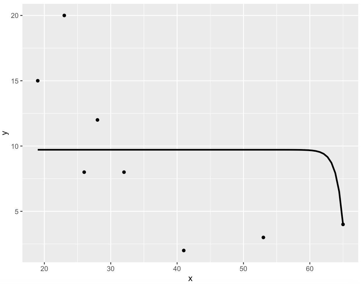
p <- ggplot(data = df, aes(x = x, y = y)) +
geom_smooth(method = "glm", se=FALSE, color="black", formula = y ~ exp(x)) +
geom_point()
p有问题的适合:
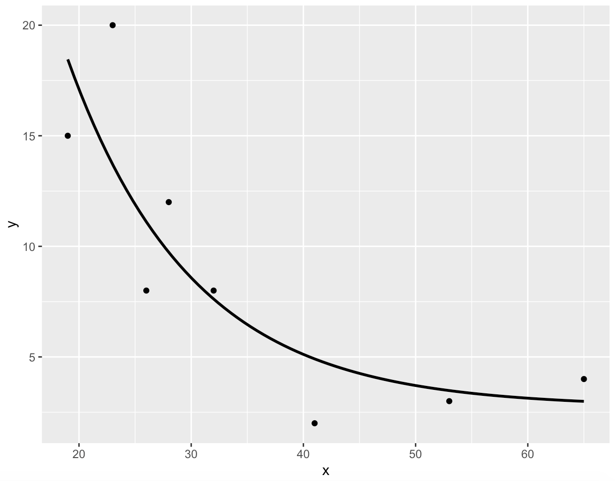
然而,如果指数内的参数是合适的,那么趋势线的形式就变得合理了:
p <- ggplot(data = df, aes(x = x, y = y)) +
  geom_smooth(method = "glm", se=FALSE, color="black", formula = y ~ exp(-0.09 * x)) +
  geom_point()

p
Stack Overflow用户
发布于 2020-05-07 05:10:51
首先,要将附加参数传递给传递给method param of geom_smooth的函数,您可以向method.args传递一个命名参数列表。
其次,你看到的问题是,glm把系数放在整个术语的前面:y ~ coef * exp(x)而不是inside:y ~ exp(coef * x),就像你想要的那样。您可以在glm之外使用优化来解决后者,但是您可以通过转换:日志链接将其融入GLM范式。这是因为它就像取你想要拟合的方程,y = exp(coef * x),并取两边的日志,所以你现在拟合log(y) = coef * x,这相当于你想要拟合的,并与GLM范例一起工作。(这忽略了拦截。它也在转换后的链接单元中结束,但是如果您愿意的话,可以很容易地将其转换回来。)
您可以在ggplot之外运行这个程序,以查看模型的外观:
df <- data.frame(
    x = c(65,53,41,32,28,26,23,19),
    y <- c(4,3,2,8,12,8,20,15)
)

bad_model <- glm(y ~ exp(x), family = gaussian(link = 'identity'), data = df)
good_model <- glm(y ~ x, family = gaussian(link = 'log'), data = df)

# this is bad
summary(bad_model)
#>
#> Call:
#> glm(formula = y ~ exp(x), family = gaussian(link = "identity"),
#>     data = df)
#>
#> Deviance Residuals:
#>     Min       1Q   Median       3Q      Max
#> -7.7143  -2.9643  -0.8571   3.0357  10.2857
#>
#> Coefficients:
#>               Estimate Std. Error t value Pr(>|t|)
#> (Intercept)  9.714e+00  2.437e+00   3.986  0.00723 **
#> exp(x)      -3.372e-28  4.067e-28  -0.829  0.43881
#> ---
#> Signif. codes:  0 '***' 0.001 '**' 0.01 '*' 0.05 '.' 0.1 ' ' 1
#>
#> (Dispersion parameter for gaussian family taken to be 41.57135)
#>
#>     Null deviance: 278.00  on 7  degrees of freedom
#> Residual deviance: 249.43  on 6  degrees of freedom
#> AIC: 56.221
#>
#> Number of Fisher Scoring iterations: 2

# this is better
summary(good_model)
#>
#> Call:
#> glm(formula = y ~ x, family = gaussian(link = "log"), data = df)
#>
#> Deviance Residuals:
#>    Min      1Q  Median      3Q     Max
#> -3.745  -2.600   0.046   1.812   6.080
#>
#> Coefficients:
#>             Estimate Std. Error t value Pr(>|t|)
#> (Intercept)  3.93579    0.51361   7.663 0.000258 ***
#> x           -0.05663    0.02054  -2.757 0.032997 *
#> ---
#> Signif. codes:  0 '***' 0.001 '**' 0.01 '*' 0.05 '.' 0.1 ' ' 1
#>
#> (Dispersion parameter for gaussian family taken to be 12.6906)
#>
#>     Null deviance: 278.000  on 7  degrees of freedom
#> Residual deviance:  76.143  on 6  degrees of freedom
#> AIC: 46.728
#>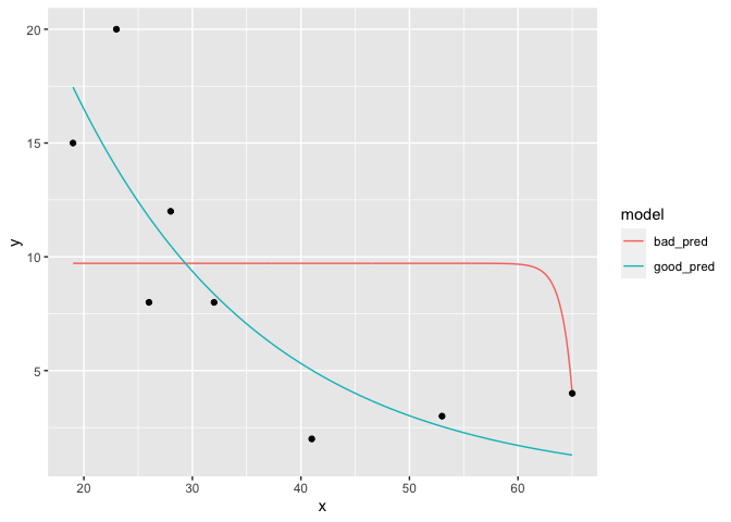
#> Number of Fisher Scoring iterations: 6在这里,您可以再现geom_smooth将要做的事情:跨域创建x值序列,并将预测用作行的y值:
# new data is a sequence across the domain of the model
new_df <- data.frame(x = seq(min(df$x), max(df$x), length = 501))

# `type = 'response'` because we want values for y back in y units
new_df$bad_pred <- predict(bad_model, newdata = new_df, type = 'response')
new_df$good_pred <- predict(good_model, newdata = new_df, type = 'response')

library(tidyr)
library(ggplot2)

new_df %>%
    # reshape to long form for ggplot
    gather(model, y, contains('pred')) %>%
    ggplot(aes(x, y)) +
    geom_line(aes(color = model)) +
    # plot original points on top
    geom_point(data = df)
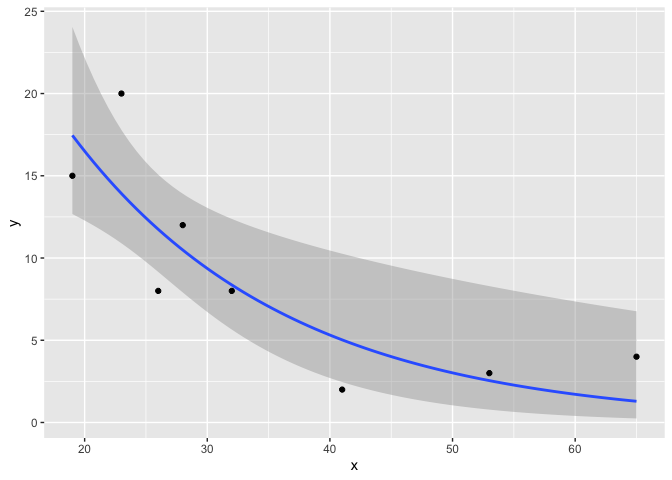
当然,让ggplot为您处理所有这些问题要容易得多:
ggplot(df, aes(x, y)) +
    geom_smooth(
        method = 'glm',
        formula = y ~ x,
        method.args = list(family = gaussian(link = 'log'))
    ) +
    geom_point()
页面原文内容由Stack Overflow提供。腾讯云小微IT领域专用引擎提供翻译支持
原文链接:
https://stackoverflow.com/questions/61648450
复制相关文章
相似问题
腾讯云开发者
