文章/答案/技术大牛

发布

社区首页 >问答首页 >如何拟合考虑不确定性的指数衰减曲线？

问如何拟合考虑不确定性的指数衰减曲线？
EN

Stack Overflow用户

提问于 2021-02-11 12:22:47

回答 1查看 766关注 0票数 4

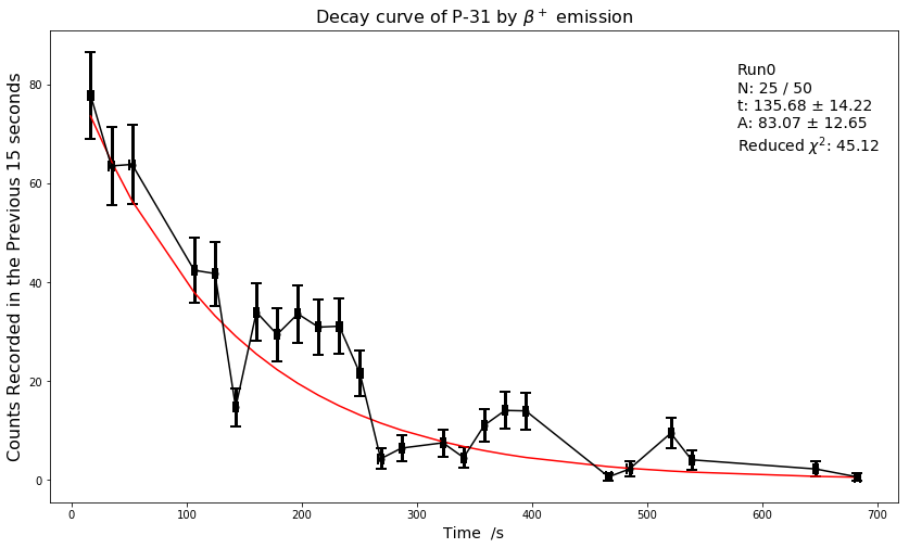
我有一些放射性衰变数据，x和y都有不确定性。图本身都很好，但我需要绘制指数衰变曲线并返回拟合的报告，以求半衰期，并将chi^2化简。

图的代码是：

 fig, ax = plt.subplots(figsize=(14, 8))
    ax.errorbar(ts, amps, xerr=2, yerr=sqrt(amps), fmt="ko-", capsize = 5, capthick= 2, elinewidth=3, markersize=5)
    plt.xlabel('Time  /s', fontsize=14)
    plt.ylabel('Counts Recorded in the Previous 15 seconds', fontsize=16)
    plt.title("Decay curve of P-31 by $β^+$ emission", fontsize=16)

我使用的模型(诚然，我对这里的编程不太自信)是：

def expdecay(x, t, A): 
     return A*exp(-x/t)

    decayresult = emodel.fit(amps, x=ts, t=150, A=140)
    ax.plot(ts, decayresult.best_fit, 'r-', label='best fit')
    
    print(decayresult.fit_report())

但我认为这并没有考虑到不确定性，只是在图表上绘制了它们。我希望它拟合指数衰减曲线，考虑了不确定因素，返回半衰期(在这种情况下t)，并用它们各自的不确定性来降低chi^2。

以下面的图片为目标，但考虑到拟合过程中的不确定性：

使用weight=1/sqrt(amps)建议和完整的数据集，我得到：

我想，这是从这些数据中得到的最佳拟合值(将chi^s降为3.89)。我希望它能给我t=150s，但是嘿，那个正在做实验。谢谢大家的帮助。

python

matplotlib

exponential

errorbar

lmfit

回答 1

Stack Overflow用户

回答已采纳

发布于 2021-02-11 16:28:08

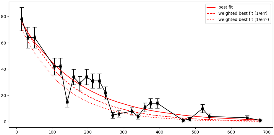
可以使用weights参数指定权重。为了给小不确定性的值赋予更多的权重，例如使用1/uncertainty。

但是，这个例子中的不确定性的问题是，它们直接依赖于振幅(uncertainty=np.sqrt(amps))的值。如果你使用这种不确定因素，它们只会将你的拟合曲线向下移动。因此，只有当你的不确定性是从某种测量中获得的真实不确定性时，这种方法才有意义。

示例：

import matplotlib.pyplot as plt
import numpy as np
import lmfit

ts = np.array([ 15,  32,  51, 106, 123, 142, 160, 177, 196, 213, 232, 249, 269, 286, 323, 340, 359, 375, 394, 466, 484, 520, 539, 645, 681])
amps = np.array([78, 64, 64, 42, 42, 15, 34, 29, 34, 31, 31, 22,  5,  6,  8,  4, 11, 14, 14,  1,  2, 10,  4,  3,  1])
emodel = lmfit.Model(lambda x,t,A: A*np.exp(-x/t))

plt.errorbar(ts, amps, xerr=2, yerr=np.sqrt(amps), fmt="ko-", capsize = 5)
plt.plot(ts, emodel.fit(amps, x=ts, t=150, A=140).best_fit, 'r-', label='best fit')
plt.plot(ts, emodel.fit(amps, x=ts, weights=1/np.sqrt(amps), t=150, A=140).best_fit, 'r--', label='weighted best fit (1/err)')
plt.plot(ts, emodel.fit(amps, x=ts, weights=1/amps, t=150, A=140).best_fit, 'r:', label='weighted best fit (1/err²)')
plt.legend()

票数 2

页面原文内容由Stack Overflow提供。腾讯云小微IT领域专用引擎提供翻译支持

原文链接：

https://stackoverflow.com/questions/66154701

复制

相似问题

问如何拟合考虑不确定性的指数衰减曲线？
EN

回答 1

Stack Overflow用户

社区

活动

圈层

关于

腾讯云开发者

热门产品

热门推荐

更多推荐

问如何拟合考虑不确定性的指数衰减曲线？EN

回答 1

Stack Overflow用户

社区

活动

圈层

关于

腾讯云开发者

热门产品

热门推荐

更多推荐

问如何拟合考虑不确定性的指数衰减曲线？
EN