
如何实现像scipy.signal.lfilter这样的过滤器
如何实现像scipy.signal.lfilter这样的过滤器
提问于 2014-01-04 04:47:49
我用python制作了一个原型,正在转换为一个iOS应用程序。不幸的是,在objective中并没有使用scipy和numpy的所有优点。所以,显然我需要从头到尾在目标C中实现一个过滤器。作为第一步,我正尝试在python中从头开始实现IIR。如果我能理解如何在python中这样做,我就可以用C语言编写它。
作为附带说明,我希望有任何关于在iOS中进行过滤的资源的建议。作为熟悉matlab和python的目标C的新手,我感到震惊的是,音频工具箱、加速框架和令人惊异的音频引擎没有与scipy.signal.filtfilt相当的功能,也没有像scipy.signal.butter这样的过滤器设计功能。
因此,在下面的代码中,我用五种方式实现了过滤器。1) scipy.signal.lfilter (用于比较),2)利用Matlab的黄油函数计算A,B,C,D矩阵的状态空间形式。3)利用scipy.signal.tf2ss计算的A,B,C,D矩阵的状态空间形式。4)直接表格I,5)直接表格II。
如您所见,使用Matlab矩阵的状态空间表单工作得很好,我可以在我的应用程序中使用它。然而,我仍然在努力理解为什么其他人工作得不太好。
import numpy as np
from scipy.signal  import butter, lfilter, tf2ss

# building the test signal, a sum of two sines;
N = 32
x = np.sin(np.arange(N)/6. * 2 * np.pi)+\
    np.sin(np.arange(N)/32. * 2 * np.pi)
x = np.append([0 for i in range(6)], x)

# getting filter coefficients from scipy
b,a = butter(N=6, Wn=0.5)

# getting matrices for the state-space form of the filter from scipy.
A_spy, B_spy, C_spy, D_spy = tf2ss(b,a)

# matrices for the state-space form as generated by matlab (different to scipy's)
A_mlb = np.array([[-0.4913, -0.5087, 0, 0, 0, 0],
        [0.5087, 0.4913, 0, 0, 0, 0],
        [0.1490, 0.4368, -0.4142, -0.5858, 0, 0],
        [0.1490, 0.4368, 0.5858, 0.4142, 0, 0],
        [0.0592, 0.1735, 0.2327, 0.5617, -0.2056, -0.7944],
        [0.0592, 0.1735, 0.2327, 0.5617, 0.7944, 0.2056]])

B_mlb = np.array([0.7194, 0.7194, 0.2107, 0.2107, 0.0837, 0.0837])

C_mlb = np.array([0.0209, 0.0613, 0.0823, 0.1986, 0.2809, 0.4262])

D_mlb = 0.0296

# getting results of scipy lfilter to test my implementation against
y_lfilter = lfilter(b, a, x)

# initializing y_df1, the result of the Direct Form I method.
y_df1 = np.zeros(6)

# initializing y_df2, the result of the Direct Form II method.
# g is an array also used in the calculation of Direct Form II
y_df2 = np.array([])
g = np.zeros(6)

# initializing z and y for the state space version with scipy matrices.
z_ss_spy = np.zeros(6)
y_ss_spy = np.array([])

# initializing z and y for the state space version with matlab matrices.
z_ss_mlb = np.zeros(6)
y_ss_mlb = np.array([])


# applying the IIR filter, in it's different implementations
for n in range(N):
    # The Direct Form I
    y_df1 = np.append(y_df1, y_df1[-6:].dot(a[:0:-1]) + x[n:n+7].dot(b[::-1]))

    # The Direct Form II
    g = np.append(g, x[n] + g[-6:].dot(a[:0:-1]))
    y_df2 = np.append(y_df2, g[-7:].dot(b[::-1]))

    # State space with scipy's matrices
    y_ss_spy = np.append(y_ss_spy, C_spy.dot(z_ss_spy) + D_spy * x[n+6])
    z_ss_spy = A_spy.dot(z_ss_spy) + B_spy * x[n+6]

    # State space with matlab's matrices
    y_ss_mlb = np.append(y_ss_mlb, C_mlb.dot(z_ss_mlb) + D_mlb * x[n+6])
    z_ss_mlb = A_mlb.dot(z_ss_mlb) + B_mlb * x[n+6]


# getting rid of the zero padding in the results
y_lfilter = y_lfilter[6:]
y_df1 = y_df1[6:]
y_df2 = y_df2[6:]


# printing the results
print "{}\t{}\t{}\t{}\t{}".format('lfilter','matlab ss', 'scipy ss', 'Direct Form I', 'Direct Form II')
for n in range(N-6):
    print "{}\t{}\t{}\t{}\t{}".format(y_lfilter[n], y_ss_mlb[n], y_ss_spy[n], y_df1[n], y_df2[n])
以及产出:
lfilter         matlab ss       scipy ss        Direct Form I   Direct Form II
0.0             0.0             0.0             0.0             0.0
0.0313965294015 0.0314090254837 0.0313965294015 0.0313965294015 0.0313965294015
0.225326252712  0.22531468279   0.0313965294015 0.225326252712  0.225326252712
0.684651781013  0.684650012268  0.0313965294015 0.733485689277  0.733485689277
1.10082931381   1.10080090424   0.0313965294015 1.45129994748   1.45129994748
0.891192957678  0.891058879496  0.0313965294015 2.00124367289   2.00124367289
0.140178897557  0.139981099035  0.0313965294015 2.17642377522   2.17642377522
-0.162384434762 -0.162488434882 0.225326252712  2.24911228252   2.24911228252
0.60258601688   0.602631573263  0.225326252712  2.69643931422   2.69643931422
1.72287292534   1.72291129518   0.225326252712  3.67851039998   3.67851039998
2.00953056605   2.00937857026   0.225326252712  4.8441925268    4.8441925268
1.20855478679   1.20823164284   0.225326252712  5.65255635018   5.65255635018
0.172378732435  0.172080718929  0.225326252712  5.88329450124   5.88329450124
-0.128647387408 -0.128763927074 0.684651781013  5.8276996139    5.8276996139
0.47311062085   0.473146568232  0.684651781013  5.97105082682   5.97105082682
1.25980235112   1.25982698592   0.684651781013  6.48492462347   6.48492462347
1.32273336715   1.32261397627   0.684651781013  7.03788646586   7.03788646586
0.428664985784  0.428426965442  0.684651781013  7.11454966484   7.11454966484
-0.724128943343 -0.724322419906 0.684651781013  6.52441390718   6.52441390718
-1.16886662032  -1.16886884238  1.10082931381   5.59188293911   5.59188293911
-0.639469994539 -0.639296371149 1.10082931381   4.83744942709   4.83744942709
0.153883055505  0.154067363252  1.10082931381   4.46863620556   4.46863620556
0.24752293493   0.247568224184  1.10082931381   4.18930262192   4.18930262192
-0.595875437915 -0.595952759718 1.10082931381   3.51735265599   3.51735265599
-1.64776590859  -1.64780228552  1.10082931381   2.29229811755   2.29229811755
-1.94352867959 -1.94338167159 0.891192957678 0.86412577159 0.86412577159Stack Overflow用户
发布于 2014-01-04 06:31:38
看看FIR维基,这个公式:
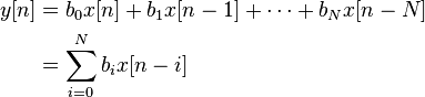
因此,首先您自己生成一个hamming窗口(我仍然在使用python,但是可以将它转换为c/cpp):
def getHammingWin(n):
    ham=[0.54-0.46*np.cos(2*np.pi*i/(n-1)) for i in range(n)]
    ham=np.asanyarray(ham)
    ham/=ham.sum()
    return ham
然后你自己的低通滤波器:
def myLpf(data, hamming):

    N=len(hamming)
    res=[]
    for n, v in enumerate(data):
        y=0
        for i in range(N):
            if n<i:
                break
            y+=hamming[i]*data[n-i]
        res.append(y)
    return np.asanyarray(res)
pass页面原文内容由Stack Overflow提供。腾讯云小微IT领域专用引擎提供翻译支持
原文链接:
https://stackoverflow.com/questions/20917019
复制相关文章
相似问题
腾讯云开发者
