
基于R(气泡图可视化)的编程
基于R(气泡图可视化)的编程
提问于 2014-10-10 05:25:32
我有一个乘客出行频率的数据集:
CountryOrigin -有40多个国家的名字
(印度、澳大利亚、中国、日本、巴丹、巴厘、新加坡)
CountryDestination -有40+国家名称(印度、澳大利亚、中国、日本、巴丹、巴厘、新加坡)
       IND   AUS   CHI   JAP   BAT   SING
 IND     0     4    10    12    24     89
 AUS    19     0    12     9     7     20
 CHI    34    56     0     2     6     18
 JAP    12    17    56     0     2      2
 SING   56    34     7     3    35      0
我需要在x轴的起源位置名称和y轴的目的地名称,频率应该表示为气泡的大小。
回答 2
Stack Overflow用户
回答已采纳
发布于 2014-10-10 06:55:03
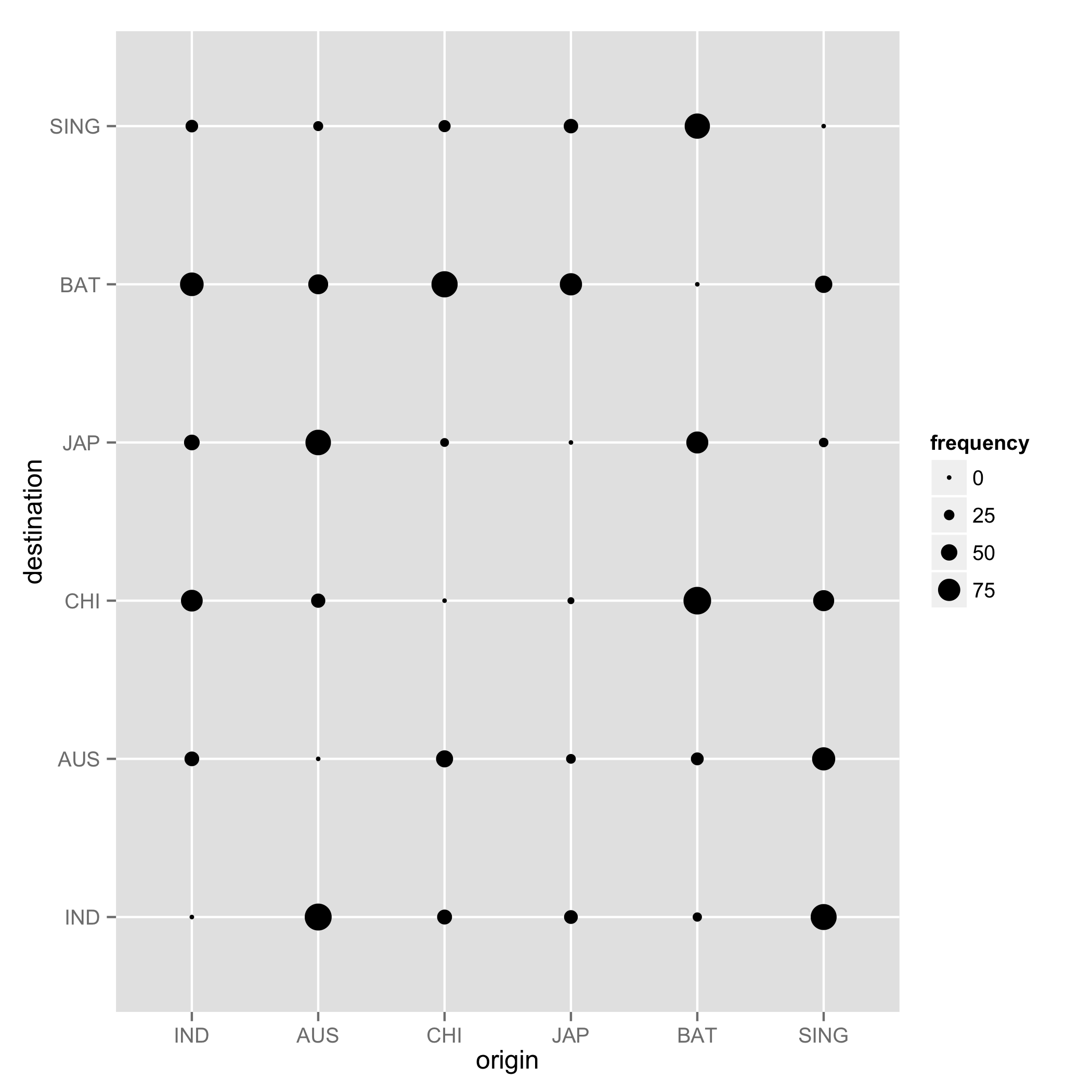
我会将ggplot2用于这些(或任何类型的)地块。让我们首先创建一些测试数据:
countries = c('IND', 'AUS', 'CHI', 'JAP', 'BAT', 'SING')
frequencies = matrix(sample(1:100, 36), 6, 6, dimnames = list(countries, countries))
diag(frequencies) = 0
然后编个故事。首先,我们必须将矩阵数据转换成适当的格式:
library(reshape2)
frequencies_df = melt(frequencies)
names(frequencies_df) = c('origin', 'destination', 'frequency')并使用ggplot2
library(ggplot2)
ggplot(frequencies_df, aes(x = origin, y = destination, size = frequencies)) + geom_point()
Stack Overflow用户
发布于 2014-10-13 15:30:55
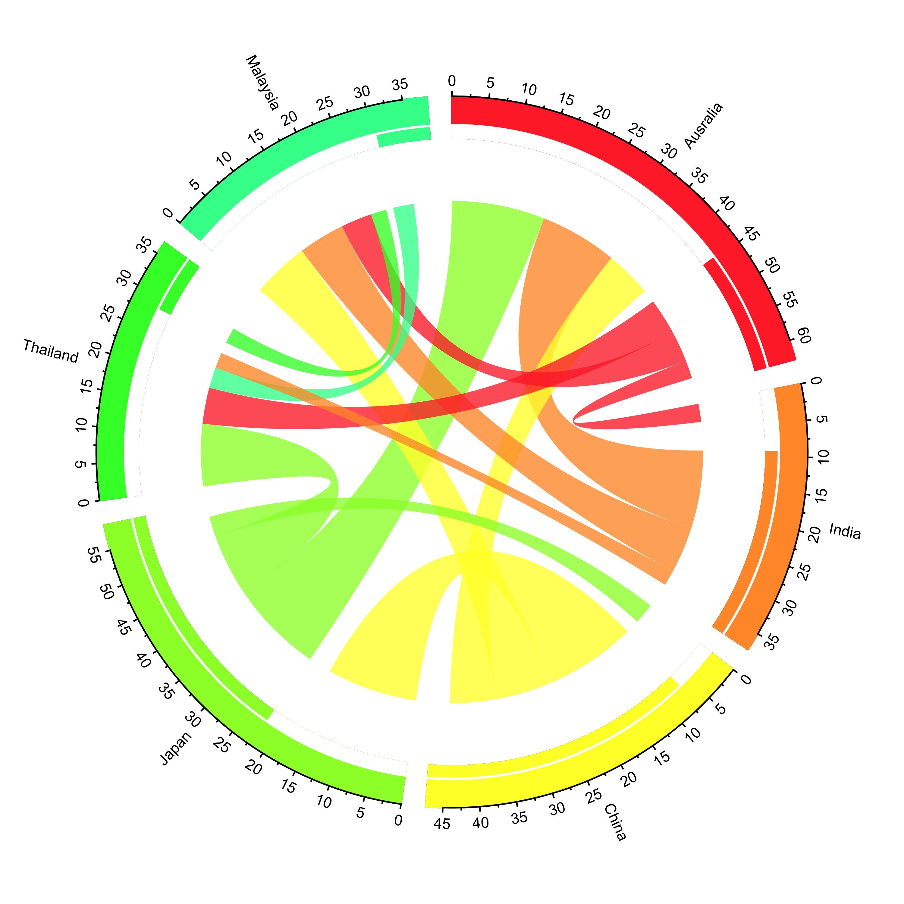
我想留下另一种方法来可视化这些数据。通过在R中使用circlize和migest包,您可以直观地看到人们是如何移动或旅行的。您需要进行大量的编码,但是如果您按照migest中的演示进行演示,仍然可以创建您想要的东西。您需要一个矩阵和一个数据框架来绘制这个数字。但是,一旦你有了他们的权利,你可以使用代码从演示。在这个例子中,你可以看到来自6个国家的人们是如何旅行的。例如,澳洲人在这些假数据中访问了日本、马来西亚和印度;三条红线到达了这些国家。如果线路更宽,那就意味着有更多的人访问了这些国家。同样,中国人访问了澳大利亚、日本和马来西亚。我把密码留在这里了。
library(circlize)
library(migest)
library(dplyr)

m <- data.frame(order = 1:6,
            country = c("Ausralia", "India", "China", "Japan", "Thailand", "Malaysia"),
            V3 = c(1, 150000, 90000, 180000, 15000, 10000),
            V4 = c(35000, 1, 10000, 12000, 25000, 8000),
            V5 = c(10000, 7000, 1, 40000, 5000, 4000),
            V6 = c(7000, 8000, 175000, 1, 11000, 18000),
            V7 = c(70000, 30000, 22000, 120000, 1, 40000),
            V8 = c(60000, 90000, 110000, 14000, 30000, 1),
            r = c(255,255,255,153,51,51),
            g = c(51, 153, 255, 255, 255, 255),
            b = c(51, 51, 51, 51, 51, 153),
            stringsAsFactors = FALSE)

### Create a data frame
df1 <- m[, c(1,2, 9:11)]

### Create a matrix
m <- m[,-(1:2)]/1e04
m <- as.matrix(m[,c(1:6)])
dimnames(m) <- list(orig = df1$country, dest = df1$country)


### Sort order of data.frame and matrix for plotting in circos

df1 <- arrange(df1, order)

df1$country <- factor(df1$country, levels = df1$country)

m <- m[levels(df1$country),levels(df1$country)]


### Define ranges of circos sectors and their colors (both of the sectors and the links)

df1$xmin <- 0

df1$xmax <- rowSums(m) + colSums(m)

n <- nrow(df1)

df1$rcol<-rgb(df1$r, df1$g, df1$b, max = 255)

df1$lcol<-rgb(df1$r, df1$g, df1$b, alpha=200, max = 255)


##
## Plot sectors (outer part)
##

par(mar=rep(0,4))

circos.clear()

### Basic circos graphic parameters
circos.par(cell.padding=c(0,0,0,0), track.margin=c(0,0.15), start.degree = 90, gap.degree =4)

### Sector details
circos.initialize(factors = df1$country, xlim = cbind(df1$xmin, df1$xmax))

### Plot sectors

circos.trackPlotRegion(ylim = c(0, 1), factors = df1$country, track.height=0.1,
                      #panel.fun for each sector
                      panel.fun = function(x, y) {
                      #select details of current sector
                      name = get.cell.meta.data("sector.index")
                      i = get.cell.meta.data("sector.numeric.index")
                      xlim = get.cell.meta.data("xlim")
                      ylim = get.cell.meta.data("ylim")

                      #text direction (dd) and adjusmtents (aa)
                      theta = circlize(mean(xlim), 1.3)[1, 1] %% 360
                      dd <- ifelse(theta < 90 || theta > 270, "clockwise", "reverse.clockwise")
                      aa = c(1, 0.5)
                      if(theta < 90 || theta > 270)  aa = c(0, 0.5)

                      #plot country labels
                      circos.text(x=mean(xlim), y=1.7, labels=name, facing = dd, cex=0.6,  adj = aa)

                      #plot main sector
                      circos.rect(xleft=xlim[1], ybottom=ylim[1], xright=xlim[2], ytop=ylim[2],
                                  col = df1$rcol[i], border=df1$rcol[i])

                      #blank in part of main sector
                      circos.rect(xleft=xlim[1], ybottom=ylim[1], xright=xlim[2]-rowSums(m)[i], ytop=ylim[1]+0.3,
                                  col = "white", border = "white")

                      #white line all the way around
                      circos.rect(xleft=xlim[1], ybottom=0.3, xright=xlim[2], ytop=0.32, col = "white", border = "white")

                      #plot axis
                      circos.axis(labels.cex=0.6, direction = "outside", major.at=seq(from=0,to=floor(df1$xmax)[i],by=5),
                                  minor.ticks=1, labels.away.percentage = 0.15)
                    })


##
## Plot links (inner part)
##

### Add sum values to df1, marking the x-position of the first links
### out (sum1) and in (sum2). Updated for further links in loop below.

df1$sum1 <- colSums(m)
df1$sum2 <- numeric(n)

### Create a data.frame of the flow matrix sorted by flow size, to allow largest flow plotted first
df2 <- cbind(as.data.frame(m),orig=rownames(m),  stringsAsFactors=FALSE)

df2 <- reshape(df2, idvar="orig", varying=list(1:n), direction="long",
           timevar="dest", time=rownames(m),  v.names = "m")

df2 <- arrange(df2,desc(m))

### Keep only the largest flows to avoid clutter
df2 <- subset(df2, m > quantile(m,0.6))

### Plot links

for(k in 1:nrow(df2)){
    #i,j reference of flow matrix
    i<-match(df2$orig[k],df1$country)
    j<-match(df2$dest[k],df1$country)

#plot link
circos.link(sector.index1=df1$country[i], point1=c(df1$sum1[i], df1$sum1[i] + abs(m[i, j])),
            sector.index2=df1$country[j], point2=c(df1$sum2[j], df1$sum2[j] + abs(m[i, j])),
            col = df1$lcol[i])

#update sum1 and sum2 for use when plotting the next link
df1$sum1[i] = df1$sum1[i] + abs(m[i, j])
df1$sum2[j] = df1$sum2[j] + abs(m[i, j])
}页面原文内容由Stack Overflow提供。腾讯云小微IT领域专用引擎提供翻译支持
原文链接:
https://stackoverflow.com/questions/26292484
复制相关文章
相似问题
腾讯云开发者
