
利用nlsLM函数寻找非线性模型的初始条件
我正在使用来自nlsLM包的minpack.lm函数来查找参数a, e和c的值,这些参数最适合于数据out。这是我的代码:
n <- seq(0, 70000, by = 1)
TR <- 0.946
b <- 2000
k <- 50000
nr <- 25
na <- 4000
nd <- 3200
d <- 0.05775
y <- d + ((TR*b)/k)*(nr/(na + nd + nr))*n
## summary(y)
out <- data.frame(n = n, y = y)
plot(out$n, out$y)
## Estimate the parameters of a nonlinear model
library(minpack.lm)
k1 <- 50000
k2 <- 5000
fit_r <- nlsLM(y ~ a*(e*n + k1*k2 + c), data=out,
start=list(a = 2e-10,
e = 6e+05,
c = 1e+07), lower = c(0, 0, 0), algorithm="port")
print(fit_r)
## summary(fit_r)
df_fit <- data.frame(n = seq(0, 70000, by = 1))
df_fit$y <- predict(fit_r, newdata = df_fit)
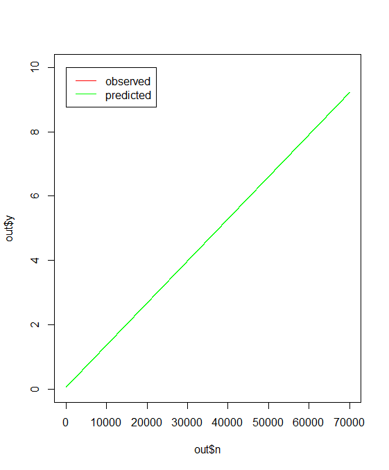
plot(out$n, out$y, type = "l", col = "red", ylim = c(0,10))
lines(df_fit$n, df_fit$y, col="green")
legend(0,ceiling(max(out$y)),legend=c("observed","predicted"), col=c("red","green"), lty=c(1,1), ncol=1)对数据的拟合似乎对初始条件非常敏感。例如:
- 对于
list(a = 2e-10, e = 6e+05, c = 1e+07),这提供了一个很好的匹配:
非线性回归模型:y~a* (e *n+ k1 * k2 + c)数据:a_c 2.221e-10 5.895e+05 9.996e+06残差平方: 3.225e-26算法“端口”,收敛信息:
par' and the solution is at mostptol‘之间的相对误差。
- 对于
list(a = 2e-01, e = 100, c = 2),这给出了一个不合适的结果:
非线性回归模型:y~a* (e *n+ k1 * k2 + c)数据:a_c 1.839e-08 1.000e+02 0.000e+00残差平方: 476410算法“端口”,收敛信息:平方和的相对误差最多为‘`ftol’。
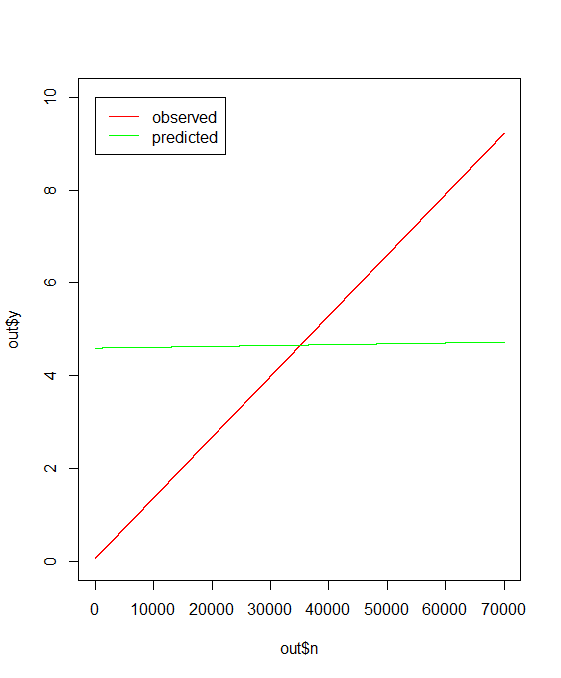
那么,是否有一种有效的方法来找到适合数据的初始条件?
编辑
我添加了下面的代码来更好地解释这个问题。该代码用于查找a、e和c的值,这些值对来自多个数据集的数据最适合。Y中的每一行对应一个数据集。通过运行代码,第三个数据集(或Y中的第3行)有一个错误消息:singular gradient matrix at initial parameter estimates.这里是代码:
TR <- 0.946
b <- 2000
k <- 50000
nr <- 25
na <- 4000
nd <- 3200
d <- 0.05775

Y <- data.frame(k1 = c(114000, 72000, 2000, 100000), k2 = c(47356, 30697, 214, 3568), n = c(114000, 72000, 2000, 100000),
           na = c(3936, 9245, 6834, 2967), nd = c(191, 2409, 2668, 2776), nr = c(57, 36, 1, 50), a = NA, e = NA, c = NA)

## Create a function to round values
roundDown <- function(x) {
  k <- floor(log10(x))
  out <- floor(x*10^(-k))*10^k
  return(out)
}

ID_line_NA <- which(is.na(Y[,c("a")]), arr.ind=TRUE)
## print(ID_line_NA)

for(i in ID_line_NA){

  print(i)

  ## Define the variable y
  seq_n <- seq(0, Y[i, c("n")], by = 1)
  y <- d + (((TR*b)/(Y[i, c("k1")]))*(Y[i, c("nr")]/(Y[i, c("na")] + Y[i, c("nd")] + Y[i, c("nr")])))*seq_n
  ## summary(y)
  out <- data.frame(n = seq_n, y = y)
  ## plot(out$n, out$y)

  ## Build the linear model to find the values of parameters that give the best fit
  mod <- lm(y ~ n, data = out)
  ## print(mod)

  ## Define initial conditions
  test_a <- roundDown(as.vector(coefficients(mod)[1])/(Y[i, c("k1")]*Y[i, c("k2")]))
  test_e <- as.vector(coefficients(mod)[2])/test_a
  test_c <- (as.vector(coefficients(mod)[1])/test_a) - (Y[i, c("k1")]*Y[i, c("k2")])

  ## Build the nonlinear model
  fit <- tryCatch( nlsLM(y ~ a*(e*n + Y[i, c("k1")]*Y[i, c("k2")] + c), data=out,
                                   start=list(a = test_a,
                                              e = test_e,
                                              c = test_c), lower = c(0, 0, 0)),
                             warning = function(w) return(1), error = function(e) return(2))
  ## print(fit)

  if(is(fit,"nls")){

    ## Plot
    tiff(paste("F:/Sources/Test_", i, ".tiff", sep=""), width = 10, height = 8, units = 'in', res = 300)
    par(mfrow=c(1,2),oma = c(0, 0, 2, 0))
    df_fit <- data.frame(n = seq_n)
    df_fit$y <- predict(fit, newdata = df_fit)
    plot(out$n, out$y, type = "l", col = "red", ylim = c(0, ceiling(max(out$y))))
    lines(df_fit$n, df_fit$y, col="green")
    dev.off()

    ## Add the parameters a, e and c in the data frame
    Y[i, c("a")] <- as.vector(coef(fit)[c("a")])
    Y[i, c("e")] <- as.vector(coef(fit)[c("e")])
    Y[i, c("c")] <- as.vector(coef(fit)[c("c")])

  } else{

    print("Error in the NLM")

  }
}那么,使用约束a > 0, e > 0, and c > 0,是否有一种有效的方法可以为nlsLM函数找到适合数据的初始条件并避免错误消息?
我添加了一些条件来定义参数a、e和c的初始条件。
利用线性模型lm(y ~ n)的结果
C=截距/a-K1*K2>0和e=斜率/a>0
,其中intercept和slope分别是lm(y ~ n)的截距和斜率。
回答 1
Stack Overflow用户
发布于 2018-09-03 23:02:24
问题不在于如何找到参数的初始值。问题是,这是一个带约束的再参数线性模型。线性模型的参数是斜率a*e和截距a*(k1 * k2 + c),因此只能有两个参数,如斜率和截距,但问题中的公式试图定义三个参数:a、c和e。
我们需要修复其中一个变量,或者,通常需要添加一个附加约束。现在,如果co是一个向量,其第一个元素是Intercept,第二个元素是线性模型的斜率
fm <- lm(y ~ n)
co <- coef(fm)
然后我们得到了方程:
co[[1]] = a*e
co[[2]] = a*(k1*k2+c)co、k1和k2是已知的,如果我们认为c是固定的,那么我们可以为a和e求解:
a = co[[2]] / (k1*k2 + c)
e = (k1 * k2 + c) * co[[1]] / co[[2]]由于co[[1]]和co[[2]]都是正的,而c必须太过,所以a和e也必然是正的,一旦我们任意修复c,就给出一个解决方案。这给出无限个a,e对,使模型最小化,每个c的非负值都有一个。注意,我们不需要为此调用nlsLM。
例如,对于c = 1e-10,我们有:
fm <- lm(y ~ n)
co <- coef(fm)

c <- 1e-10
a <- co[[2]] / (k1*k2 + c)
e <- (k1 * k2 + c) * co[[1]] / co[[2]]
a; e
## [1] 5.23737e-13
## [1] 110265261628请注意,由于系数之间的幅值差异很大,可能存在数值问题;然而,如果我们增加c,会增加e,降低a,使标度变得更糟,那么问题中给出的这个问题的参数化似乎具有固有的不好的数值尺度。
请注意,所有这些都不需要运行nlsLM来获得最佳系数;但是,由于缩放性不好,可能仍然有可能在一定程度上改进答案。
co <- coef(lm(y ~ n))
c <- 1e-10
a <- co[[2]] / (k1*k2 + c)
e <- (k1 * k2 + c) * co[[1]] / co[[2]]
nlsLM(y ~ a * (e * n + k1 * k2 + c), start = list(a = a, e = e), lower = c(0, 0))
这意味着:
Nonlinear regression model
  model: y ~ a * (e * n + k1 * k2 + c)
   data: parent.frame()
        a         e
2.310e-10 5.668e+05
 residual sum-of-squares: 1.673e-26

Number of iterations to convergence: 12
Achieved convergence tolerance: 1.49e-08https://stackoverflow.com/questions/52156675
复制相似问题
腾讯云开发者
