
如何设置curve_fit的初始值,以找到最佳的优化,而不仅仅是局部优化?
我试图拟合一个幂律函数,并为了找到最佳的拟合参数。但是,我发现,如果参数的初始猜测不同,则“最佳匹配”输出是不同的。除非我找到正确的初始猜测,否则我可以得到最佳的优化,而不是局部优化。有没有办法找出合适的初步猜测?下面列出了我的代码。请随时输入。谢谢!
import numpy as np
import pandas as pd
from scipy.optimize import curve_fit
import matplotlib.pyplot as plt
%matplotlib inline

# power law function
def func_powerlaw(x,a,b,c):
    return a*(x**b)+c

test_X = [1.0,2,3,4,5,6,7,8,9,10]
test_Y =[3.0,1.5,1.2222222222222223,1.125,1.08,1.0555555555555556,1.0408163265306123,1.03125, 1.0246913580246915,1.02]

predict_Y = []
for x in test_X:
    predict_Y.append(2*x**-2+1)
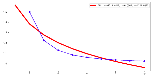
如果我与默认的初始猜测对齐,那么p0 = 1,1,1
popt, pcov = curve_fit(func_powerlaw, test_X[1:], test_Y[1:], maxfev=2000)


plt.figure(figsize=(10, 5))
plt.plot(test_X, func_powerlaw(test_X, *popt),'r',linewidth=4, label='fit: a=%.4f, b=%.4f, c=%.4f' % tuple(popt))
plt.plot(test_X[1:], test_Y[1:], '--bo')
plt.plot(test_X[1:], predict_Y[1:], '-b')
plt.legend()
plt.show()
匹配如下,这并不是最合适的。
如果我将初始猜测改为p0 = 0.5,0.5,0.5
popt, pcov = curve_fit(func_powerlaw, test_X[1:], test_Y[1:], p0=np.asarray([0.5,0.5,0.5]), maxfev=2000)我能得到最合适的
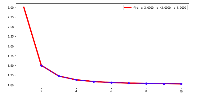
?
由于我需要运行数千到甚至百万的幂律函数,使用@James的方法太昂贵了。那么,除了curve_fit之外,还有什么方法是合适的呢?如滑雪,np.linalg.lstsq等。
回答 3
Stack Overflow用户
发布于 2018-09-16 19:48:08
下面是使用scipy.optimize.differential_evolution遗传算法的示例代码,以及您的数据和方程。本模块使用拉丁超立方体算法确保对参数空间进行彻底搜索,因此需要搜索范围--在本例中,这些边界基于数据的最大值和最小值。对于其他问题,如果您知道所期望的参数值的范围,则可能需要提供不同的搜索范围。
import numpy, scipy, matplotlib
import matplotlib.pyplot as plt
from scipy.optimize import curve_fit
from scipy.optimize import differential_evolution
import warnings

# power law function
def func_power_law(x,a,b,c):
    return a*(x**b)+c

test_X = [1.0,2,3,4,5,6,7,8,9,10]
test_Y =[3.0,1.5,1.2222222222222223,1.125,1.08,1.0555555555555556,1.0408163265306123,1.03125, 1.0246913580246915,1.02]


# function for genetic algorithm to minimize (sum of squared error)
def sumOfSquaredError(parameterTuple):
    warnings.filterwarnings("ignore") # do not print warnings by genetic algorithm
    val = func_power_law(test_X, *parameterTuple)
    return numpy.sum((test_Y - val) ** 2.0)


def generate_Initial_Parameters():
    # min and max used for bounds
    maxX = max(test_X)
    minX = min(test_X)
    maxY = max(test_Y)
    minY = min(test_Y)
    maxXY = max(maxX, maxY)

    parameterBounds = []
    parameterBounds.append([-maxXY, maxXY]) # seach bounds for a
    parameterBounds.append([-maxXY, maxXY]) # seach bounds for b
    parameterBounds.append([-maxXY, maxXY]) # seach bounds for c

    # "seed" the numpy random number generator for repeatable results
    result = differential_evolution(sumOfSquaredError, parameterBounds, seed=3)
    return result.x

# generate initial parameter values
geneticParameters = generate_Initial_Parameters()

# curve fit the test data
fittedParameters, pcov = curve_fit(func_power_law, test_X, test_Y, geneticParameters)

print('Parameters', fittedParameters)

modelPredictions = func_power_law(test_X, *fittedParameters)

absError = modelPredictions - test_Y

SE = numpy.square(absError) # squared errors
MSE = numpy.mean(SE) # mean squared errors
RMSE = numpy.sqrt(MSE) # Root Mean Squared Error, RMSE
Rsquared = 1.0 - (numpy.var(absError) / numpy.var(test_Y))
print('RMSE:', RMSE)
print('R-squared:', Rsquared)

print()


##########################################################
# graphics output section
def ModelAndScatterPlot(graphWidth, graphHeight):
    f = plt.figure(figsize=(graphWidth/100.0, graphHeight/100.0), dpi=100)
    axes = f.add_subplot(111)

    # first the raw data as a scatter plot
    axes.plot(test_X, test_Y,  'D')

    # create data for the fitted equation plot
    xModel = numpy.linspace(min(test_X), max(test_X))
    yModel = func_power_law(xModel, *fittedParameters)

    # now the model as a line plot
    axes.plot(xModel, yModel)

    axes.set_xlabel('X Data') # X axis data label
    axes.set_ylabel('Y Data') # Y axis data label

    plt.show()
    plt.close('all') # clean up after using pyplot

graphWidth = 800
graphHeight = 600
ModelAndScatterPlot(graphWidth, graphHeight)Stack Overflow用户
发布于 2018-09-17 20:41:55
没有简单的答案:如果有,它将在curve_fit中实现,然后它就不需要向您询问起点了。一种合理的方法是首先对齐次模型y = a*x**b进行拟合。假设正y(通常是幂律时的情况),这可以用一种粗略和快速的方式完成:在对数标度上,log(y) = log(a) + b*log(x)是线性回归,可以用np.linalg.lstsq求解。这给了log(a)和b的候选;使用这种方法的c的候选是0。
test_X = np.array([1.0,2,3,4,5,6,7,8,9,10])
test_Y = np.array([3.0,1.5,1.2222222222222223,1.125,1.08,1.0555555555555556,1.0408163265306123,1.03125, 1.0246913580246915,1.02])

rough_fit = np.linalg.lstsq(np.stack((np.ones_like(test_X), np.log(test_X)), axis=1), np.log(test_Y))[0]
p0 = [np.exp(rough_fit[0]), rough_fit[1], 0]
其结果是你在第二张图片中看到了很好的契合。
顺便说一句,最好立即将test_X作为一个NumPy数组。否则,首先将X[1:]切片,这会将NumPy转换为整数数组,然后用负指数抛出一个错误。(我认为1.0的目的是使它成为一个浮点数数组?这就是应该使用dtype=np.float参数的地方。)
Stack Overflow用户
发布于 2018-09-18 01:10:22
除了非常精细的答案,从欢迎到堆栈溢出,“没有简单的,通用的方法和詹姆斯菲利普斯的差异进化往往有助于找到好的起点(甚至好的解决方案!)如果比curve_fit()慢一些的话,请允许我单独给出一个你可能觉得有帮助的答案。
首先,curve_fit()默认为任何参数值这一事实是令人心碎的坏主意。这种行为是没有道理的,您和其他人都应该将参数的默认值视为curve_fit()实现中的严重错误,并假装不存在此缺陷。从未相信这些违约是合理的。
从简单的数据图来看,很明显,a=1, b=1, c=1是非常非常糟糕的起始值。函数衰变,所以b < 0。实际上,如果您从a=1, b=-1, c=1开始,您就会找到正确的解决方案。
这也可能有助于对参数设定合理的界限。即使设置(-100,100)的c界限也可能有所帮助。与b的符号一样,我认为您可以从简单的数据图中看到这个边界。当我针对您的问题尝试这样做时,如果初始值是c,则对b=0或b=-5不起作用,但对于b=0或b=-5则没有帮助。
更重要的是,尽管您在图中打印了最适合的参数popt,但是没有打印pcov中所包含的变量之间的不确定性或相关性,因此您对结果的解释是不完整的。如果你看过这些值,你就会发现,从b=1开始,不仅会导致糟糕的值,还会导致参数中的巨大不确定性和非常、非常高的相关性。这正好告诉你,它找到了一个糟糕的解决方案。不幸的是,从pcov返回curve_fit并不容易。
请允许我推荐lmfit (https://lmfit.github.io/lmfit-py/) (免责声明:我是首席开发人员)。在其他特性中,此模块强制您提供非默认的起始值,并且更容易获得更完整的报表。对于您的问题,即使是从a=1, b=1, c=1开始,也会给出一个更有意义的指示:
from lmfit import Model
mod = Model(func_powerlaw)
params = mod.make_params(a=1, b=1, c=1)
ret = mod.fit(test_Y[1:], params, x=test_X[1:])
print(ret.fit_report())
打印出来:
[[Model]]
    Model(func_powerlaw)
[[Fit Statistics]]
    # fitting method   = leastsq
    # function evals   = 1318
    # data points      = 9
    # variables        = 3
    chi-square         = 0.03300395
    reduced chi-square = 0.00550066
    Akaike info crit   = -44.4751740
    Bayesian info crit = -43.8835003
[[Variables]]
    a: -1319.16780 +/- 6892109.87 (522458.92%) (init = 1)
    b:  2.0034e-04 +/- 1.04592341 (522076.12%) (init = 1)
    c:  1320.73359 +/- 6892110.20 (521839.55%) (init = 1)
[[Correlations]] (unreported correlations are < 0.100)
    C(a, c) = -1.000
    C(b, c) = -1.000
C(a, b) = 1.000那是a = -1.3e3 +/- 6.8e6 --定义不太清楚!此外,所有参数都是完全相关的。
将b的初始值更改为-0.5:
params = mod.make_params(a=1, b=-0.5, c=1) ## Note !
ret = mod.fit(test_Y[1:], params, x=test_X[1:])
print(ret.fit_report())
给出
[[Model]]
    Model(func_powerlaw)
[[Fit Statistics]]
    # fitting method   = leastsq
    # function evals   = 31
    # data points      = 9
    # variables        = 3
    chi-square         = 4.9304e-32
    reduced chi-square = 8.2173e-33
    Akaike info crit   = -662.560782
    Bayesian info crit = -661.969108
[[Variables]]
    a:  2.00000000 +/- 1.5579e-15 (0.00%) (init = 1)
    b: -2.00000000 +/- 1.1989e-15 (0.00%) (init = -0.5)
    c:  1.00000000 +/- 8.2926e-17 (0.00%) (init = 1)
[[Correlations]] (unreported correlations are < 0.100)
    C(a, b) = -0.964
    C(b, c) = -0.880
    C(a, c) =  0.769
这有点好点。
总之,初始值总是重要的,其结果不仅是最佳拟合值,而且还包括不确定性和相关性。
https://stackoverflow.com/questions/52356128
复制相似问题
腾讯云开发者

Copyright © 2013 - 2026 Tencent Cloud. All Rights Reserved. 腾讯云 版权所有
深圳市腾讯计算机系统有限公司 ICP备案/许可证号:粤B2-20090059  粤公网安备44030502008569号
腾讯云计算(北京)有限责任公司 京ICP证150476号 | 京ICP备11018762号