
傅里叶级数拟合Python
傅里叶级数拟合Python
提问于 2018-09-26 19:34:45
我有一些数据,我想要拟合使用傅里叶级数2,3,或4度。
当堆栈溢出的这问题和答案接近我想要使用tau做的时候,他们已经将它们的系数预先定义为τ= 0.045。我想要我的拟合找到可能的系数(a0,w1,w2,w3等),95%的置信区间,就像傅里叶级数的MATLAB曲线拟合等价。我看到的另一个选项是使用级数从同情,但是这个函数只使用适合定义函数的符号参数,而不是原始数据。
( 1) fourier_series是否有一种方法可以接收原始数据,而不是使用这个库的函数或其他工作?
2)或对有多个未知数(系数)的数据进行拟合。
回答 5
Stack Overflow用户
回答已采纳
发布于 2018-09-28 12:53:29
如果您愿意的话,您可以非常接近sympy代码来进行数据拟合,使用我为此目的编写的称为symfit的包。它基本上使用scipy接口包装sympy。使用symfit,您可以执行如下操作:
from symfit import parameters, variables, sin, cos, Fit
import numpy as np
import matplotlib.pyplot as plt

def fourier_series(x, f, n=0):
    """
    Returns a symbolic fourier series of order `n`.

    :param n: Order of the fourier series.
    :param x: Independent variable
    :param f: Frequency of the fourier series
    """
    # Make the parameter objects for all the terms
    a0, *cos_a = parameters(','.join(['a{}'.format(i) for i in range(0, n + 1)]))
    sin_b = parameters(','.join(['b{}'.format(i) for i in range(1, n + 1)]))
    # Construct the series
    series = a0 + sum(ai * cos(i * f * x) + bi * sin(i * f * x)
                     for i, (ai, bi) in enumerate(zip(cos_a, sin_b), start=1))
    return series

x, y = variables('x, y')
w, = parameters('w')
model_dict = {y: fourier_series(x, f=w, n=3)}
print(model_dict)
这将打印我们想要的符号模型:
{y: a0 + a1*cos(w*x) + a2*cos(2*w*x) + a3*cos(3*w*x) + b1*sin(w*x) + b2*sin(2*w*x) + b3*sin(3*w*x)}接下来,我将把它放在一个简单的step函数中,向您展示它是如何工作的:
# Make step function data
xdata = np.linspace(-np.pi, np.pi)
ydata = np.zeros_like(xdata)
ydata[xdata > 0] = 1
# Define a Fit object for this model and data
fit = Fit(model_dict, x=xdata, y=ydata)
fit_result = fit.execute()
print(fit_result)

# Plot the result
plt.plot(xdata, ydata)
plt.plot(xdata, fit.model(x=xdata, **fit_result.params).y, color='green', ls=':')
这将打印:
Parameter Value        Standard Deviation
a0        5.000000e-01 2.075395e-02
a1        -4.903805e-12 3.277426e-02
a2        5.325068e-12 3.197889e-02
a3        -4.857033e-12 3.080979e-02
b1        6.267589e-01 2.546980e-02
b2        1.986491e-02 2.637273e-02
b3        1.846406e-01 2.725019e-02
w         8.671471e-01 3.132108e-02
Fitting status message: Optimization terminated successfully.
Number of iterations:   44
Regression Coefficient: 0.9401712713086535
并产生以下情节:
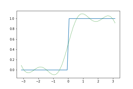
就这么简单!剩下的留给你去想象。有关更多信息,您可以找到这里的文件。
Stack Overflow用户
发布于 2018-09-27 20:22:20
我认为使用MATLAB调用python上的这函数来完成所有繁重的工作可能会更容易一些,而不是处理所有同情和参与的细节。
我的解决办法如下:
- 安装matlab和拟合函数工具箱
- 通过在extern/engines/python下的matlab根文件夹中运行
python setup.py install来安装python的matlab引擎。注意:它只适用于python 2.7、3.5和3.6 - 使用以下代码: 将matlab.engine导入np = matlab.engine.start_matlab() eng.evalc("idx =transpose(1:{})“.format(len(Diff)eng.工作区‘y’=eng.transpose(eng.cell2mat(diff.tolist() eng.evalc("f = fit(idx,y,'fourier3')") y_f = eng.evalc("f(idx)").replace('ans =','') y_f = np.fromstring(y_f,dtype=float,sep='\n')
几个注意事项:
eng.workspace['myVariable']是使用python结果声明matlab变量,这些结果以后可以通过evalc调用。eng.evalc在表单'ans =.‘中返回一个字符串- 这段代码中的
diff只是一些数据和它的最小二乘线之间的区别,它是序列类型的。 - Python列表相当于MATLAB中的单元格类型。
Stack Overflow用户
发布于 2018-09-27 07:14:08
这是我最近使用的简单代码。我知道频率,所以这是稍微修改,以适应它。不过,最初的猜测一定很好(我认为)。另一方面,有几种很好的方法来获得基频。
import numpy as np
from scipy.optimize import leastsq


def make_sine_graph( params, xData):
    """
    take amplitudes A and phases P in form [ A0, A1, A2, ..., An, P0, P1,..., Pn ]
    and construct function f = A0 sin( w t + P0) + A1 sin( 2 w t + Pn ) + ... + An sin( n w t + Pn )
    and return f( x )
    """
    fr = params[0]
    npara = params[1:]
    lp =len( npara )
    amps = npara[ : lp // 2 ]
    phases = npara[ lp // 2 : ]
    fact = range(1, lp // 2 + 1 )
    return [ sum( [ a * np.sin( 2 * np.pi * x * f * fr + p ) for a, p, f in zip( amps, phases, fact ) ] ) for x in xData ]

def sine_residuals( params , xData, yData):
    yTh = make_sine_graph( params, xData )
    diff = [ y -  yt for y, yt in zip( yData, yTh ) ]
    return diff

def sine_fit_graph( xData, yData, freqGuess=100., sineorder = 3 ):
    aStart = sineorder * [ 0 ]
    aStart[0] = max( yData )
    pStart = sineorder * [ 0 ]
    result, _ = leastsq( sine_residuals, [ freqGuess ] + aStart + pStart, args=( xData, yData ) )
    return result


if __name__ == '__main__':
    import matplotlib.pyplot as plt
    timeList = np.linspace( 0, .1, 777 )
    signalList = make_sine_graph( [  113.7 ] + [1,.5,-.3,0,.1, 0,.01,.02,.03,.04], timeList )

    result = sine_fit_graph( timeList, signalList, freqGuess=110., sineorder = 3 )
    print result
    fitList =  make_sine_graph( result, timeList )
    fig = plt.figure()
    ax = fig.add_subplot( 1, 1 ,1 )
    ax.plot( timeList, signalList )
    ax.plot( timeList, fitList, '--' )
    plt.show()
提供
<< [ 1.13699742e+02  9.99722859e-01 -5.00511764e-01  3.00772260e-01
     1.04248878e-03 -3.13050074e+00 -3.12358208e+00 ]
页面原文内容由Stack Overflow提供。腾讯云小微IT领域专用引擎提供翻译支持
原文链接:
https://stackoverflow.com/questions/52524919
复制相关文章
相似问题
腾讯云开发者
