
Matlab和Python中fmin和fminsearch结果的差异
我的目标是对一些衰变数据(通过CPMG进行核磁共振T2衰变)进行反拉普拉斯变换。为此,我们得到了CONTIN算法。该算法为改编自Matlab由Iari-Gabriel马里诺算法,运行良好。我想将这段代码改编成Python。问题的核心是scipy.optimize.fmin,它不像Matlab的fminsearch那样最小化均方偏差。后者的结果是一个很好的最小化,而前者没有。
我已经用Python和最初的Matlab逐行遍历了我的适应代码。我检查了每一个矩阵和每个输出。我用它来确定临界点在fmin中。我也尝试过scipy.optimize.minimize和其他最小化算法,但是没有一个算法给出了非常满意的结果。
我已经为Python和Matlab制作了两个MWE,以使它能够被所有人复制。实例数据是从matlab函数的文档中得到的。抱歉,如果这是长代码,但我不知道如何在不牺牲可读性和清晰度的情况下缩短它。我试着让线条尽可能地匹配。在Windows8.1上,我使用Python3.7.3,ciplyv1.3.0,numpy 1.16.2,Matlab R2018b。这是一个相对较新的Anaconda安装(<2个月)。
我的代码:
import numpy as np
from scipy.optimize import fmin
import matplotlib.pyplot as plt

def msd(g, y, A, alpha, R, w, constraints):
    """ msd: mean square deviation. This is the function to be minimized by fmin"""
    if 'zero_at_extremes' in constraints:
        g[0] = 0
        g[-1] = 0
    if 'g>0' in constraints:
        g = np.abs(g)

    r = np.diff(g, axis=0, n=2)
    yfit = A @ g
    # Sum of weighted square residuals
    VAR = np.sum(w * (y - yfit) ** 2)
    # Regularizor
    REG = alpha ** 2 * np.sum((r - R @ g) ** 2)
    # output to be minimized
    return VAR + REG

# Objective: match this distribution
g0 = np.array([0, 0, 10.1625, 25.1974, 21.8711, 1.6377, 7.3895, 8.736, 1.4256, 0, 0]).reshape((-1, 1))
s0 = np.logspace(-3, 6, len(g0)).reshape((-1, 1))
t = np.linspace(0.01, 500, 100).reshape((-1, 1))
sM, tM = np.meshgrid(s0, t)
A = np.exp(-tM / sM)
np.random.seed(1)
# Creates data from the initial distribution with some random noise.
data = (A @ g0) + 0.07 * np.random.rand(t.size).reshape((-1, 1))

# Parameters and function start
alpha = 1E-2  # regularization parameter
s = np.logspace(-3, 6, 20).reshape((-1, 1)) # x of the ILT
g0 = np.ones(s.size).reshape((-1, 1))        # guess of y of ILT
y = data                                    # noisy data
options = {'maxiter':1e8, 'maxfun':1e8}     # for the fmin function
constraints=['g>0', 'zero_at_extremes']     # constraints for the MSD function
R=np.zeros((len(g0) - 2, len(g0)), order='F')  # Regularizor
w=np.ones(y.reshape(-1, 1).size).reshape((-1, 1)) # Weights
sM, tM = np.meshgrid(s, t, indexing='xy')
A = np.exp(-tM/sM)
g0 = g0 * y.sum() / (A @ g0).sum()  # Makes a "better guess" for the distribution, according to algorithm

print('msd of input data:\n', msd(g0, y, A, alpha, R, w, constraints))

for i in range(5):  # Just for testing. If this is extremely high, ~1000, it's still bad.
    g = fmin(func=msd,
             x0 = g0,
             args=(y, A, alpha, R, w, constraints),
             **options,
             disp=True)[:, np.newaxis]
    msdfit = msd(g, y, A, alpha, R, w, constraints)
    if 'zero_at_extremes' in constraints:
            g[0] = 0
            g[-1] = 0
    if 'g>0' in constraints:
            g = np.abs(g)

    g0 = g

print('New guess', g)
print('Final msd of g', msdfit)

# Visualize the fit
plt.plot(s, g, label='Initial approximation')
plt.plot(np.logspace(-3, 6, 11), np.array([0, 0, 10.1625, 25.1974, 21.8711, 1.6377, 7.3895, 8.736, 1.4256, 0, 0]), label='Distribution to match')
plt.xscale('log')
plt.legend()
plt.show()
Matlab:
% Objective: match this distribution
g0 = [0 0 10.1625 25.1974 21.8711 1.6377 7.3895 8.736 1.4256 0 0]';
s0  = logspace(-3,6,length(g0))';
t = linspace(0.01,500,100)';
[sM,tM] = meshgrid(s0,t);
A = exp(-tM./sM);
rng(1);
% Creates data from the initial distribution with some random noise.
data = A*g0 + 0.07*rand(size(t));

% Parameters and function start
alpha = 1e-2; % regularization parameter
s = logspace(-3,6,20)'; % x of the ILT
g0 = ones(size(s)); % initial guess of y of ILT
y = data; % noisy data
options = optimset('MaxFunEvals',1e8,'MaxIter',1e8); % constraints for fminsearch
constraints = {'g>0','zero_at_the_extremes'}; % constraints for MSD
R = zeros(length(g0)-2,length(g0));
w = ones(size(y(:)));
[sM,tM] = meshgrid(s,t);
A = exp(-tM./sM);
g0 = g0*sum(y)/sum(A*g0); % Makes a "better guess" for the distribution

disp('msd of input data:')
disp(msd(g0, y, A, alpha, R, w, constraints))

for k = 1:5
    [g,msdfit] = fminsearch(@msd,g0,options,y,A,alpha,R,w,constraints);
    if ismember('zero_at_the_extremes',constraints)
        g(1) = 0;
        g(end) = 0;
    end
    if ismember('g>0',constraints)
        g = abs(g);
    end
    g0 = g;
end

disp('New guess')
disp(g)
disp('Final msd of g')
disp(msdfit)

% Visualize the fit
semilogx(s, g)
hold on
semilogx(logspace(-3,6,11), [0 0 10.1625 25.1974 21.8711 1.6377 7.3895 8.736 1.4256 0 0])
legend('First approximation', 'Distribution to match')
hold off
function out = msd(g,y,A,alpha,R,w,constraints)
% msd: The mean square deviation; this is the function
% that has to be minimized by fminsearch

% Constraints and any 'a priori' knowledge
if ismember('zero_at_the_extremes',constraints)
    g(1) = 0;
    g(end) = 0;
end
if ismember('g>0',constraints)
    g = abs(g); % must be g(i)>=0 for each i
end
r = diff(diff(g(1:end))); % second derivative of g
yfit = A*g;
% Sum of weighted square residuals
VAR = sum(w.*(y-yfit).^2);
% Regularizor
REG = alpha^2 * sum((r-R*g).^2);
% Output to be minimized
out = VAR+REG;
end
下面是Python中的优化

下面是Matlab中的优化
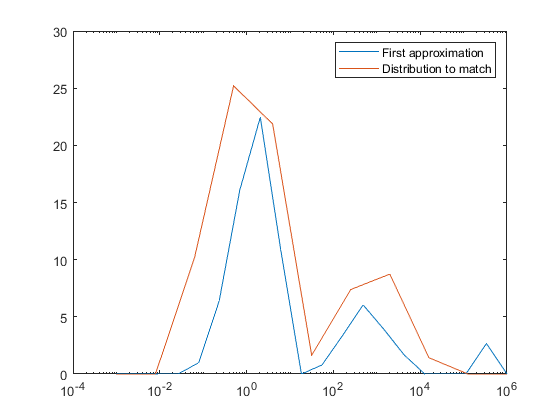
在启动前,我已经检查了g0的MSD输出,两者都给出了2651的值。最小化后,Python上升到4547,Matlab下降到0.1381。
我认为问题是以下之一。它在我的实现中,也就是说,我错误地使用了fmin,或者还有其他的段落我弄错了,但是我想不出是什么。当MSD随极小化函数减小时,MSD会增加,这是很糟糕的。阅读文档,the实现与Matlab的不同(他们使用Lagarias,根据他们的文件中描述的Nelder方法),而the使用原始的Nelder )。也许这会对你有很大的影响?或者我最初的猜测对席比的算法来说太糟糕了?
回答 1
Stack Overflow用户
发布于 2021-04-08 17:18:44
所以,很长一段时间以来,我发布了这篇文章,但我想分享我最后学习和做的事情。
CPMG数据的Laplace逆变换有点用词不当,更恰当地称为单纯反演。一般的问题是求解第一类Fredholm积分。其中一种方法是Tikhonov正则化方法。结果,您可以很容易地使用numpy来描述这个问题,并用一个can包来解决它,所以我不必用它“重新发明”轮子。
我使用了在这个岗位上显示的解决方案,这里的名称反映了该解决方案。
def tikhonov_regularized_inversion(
    kernel: np.ndarray, alpha: float, data: np.ndarray
) -> np.ndarray:
    data = data.reshape(-1, 1)
    I = alpha * np.eye(*kernel.shape)
    C = np.concatenate([kernel, I], axis=0)
    d = np.concatenate([data, np.zeros_like(data)])
x, _ = nnls(C, d.flatten())这里,kernel是一个包含所有可能的指数衰减曲线的矩阵,我的解判断每个衰减曲线在我收到的数据中的贡献。首先,我将数据堆叠成一个列,然后用零填充它,创建向量d。然后,我将内核堆在包含正则化参数alpha的对角线矩阵的顶部,该矩阵与内核大小相同。最后,我将方便的nnls称为scipy.optimize中的非负最小二乘求解器。这是因为没有理由有消极的贡献,只有没有贡献。
这解决了我的问题,它既快捷又方便。
https://stackoverflow.com/questions/57276125
复制相似问题
腾讯云开发者

Copyright © 2013 - 2026 Tencent Cloud. All Rights Reserved. 腾讯云 版权所有
深圳市腾讯计算机系统有限公司 ICP备案/许可证号:粤B2-20090059 ![]() 粤公网安备44030502008569号
粤公网安备44030502008569号
腾讯云计算(北京)有限责任公司 京ICP证150476号 | 京ICP备11018762号