Python版SCENIC转录因子分析（四）一文就够了

生信技能树

发布于 2023-02-27 21:17:34

5.1K0

发布于 2023-02-27 21:17:34

我前期写了一些关于pySCENIC的笔记，包括：

在升级了pySCENIC后，发现转录因子数据库更新了。因此本文基于更新后的转录因子数据库，再次记录了从软件部署到pySCENIC的运行，最后进行可视化的详细笔记，希望对大家有所帮助，少走弯路。

转录因子 (transcription factors, TFs) 是直接作用于基因组，与特定DNA序列结合 (TFBS/motif) ，调控DNA转录过程的一类蛋白质。转录因子可以调节基因组DNA开放性、募集RNA聚合酶进行转录过程、募集辅助因子调节特定的转录阶段，调控诸多生命进程，诸如免疫反应、发育模式等。因此，分析转录因子表达及其调控活性对于解析复杂生命活动具有重要意义。

SCENIC（single-cell regulatory network inference and clustering）是一个基于共表达和motif分析，计算单细胞转录组数据基因调控网络重建以及细胞状态鉴定的方法。在输入单细胞基因表达量矩阵后，SCENIC经过以下三个步骤完成转录因子分析：

第一步，GENIE3（随机森林)/GRNBoost (Gradient Boosting) 推断转录因子与候选靶基因之间的共表达模块，每个模块包含一个转录因子及其靶基因，纯粹基于共表达；
第二步，RcisTatget分析每个共表达模块中的基因，以鉴定enriched motifs，仅保留TF motif富集的模块和targets，构建TF-targets网络，每个TF及其潜在的直接targets gene被称作一个调节因子（Regulons）；
第三步，AUCelll计算调节因子（Regulons）的活性，这将确定Regulon在哪些细胞中处于“打开”状态。

Python版本的优势是速度快，难点是安装比较麻烦，笔者建议用Conda进行按照。

Step0.软件安装：

安装主要有三种方法docker，conda和Singularity（这里我使用conda）：

（2）conda安装

注意python版本python=3.7

# 需要一些依赖
conda create -n pyscenic python=3.7 
conda activate pyscenic 

mamba install -y numpy scanpy
mamba install -y -c anaconda cytoolz

pip install pyscenic

（3）数据库配置

转录因子分析还需要自行下载最新更新的数据库（https://resources.aertslab.org/cistarget/databases/）：

数据库储存在/data/index_genome/cisTarget_databases/

mkdir  /data/index_genome/cisTarget_databases/
cd /data/index_genome/cisTarget_databases/

下载数据库：

人的：

cat >download.bash
##1, For human:
wget -c https://resources.aertslab.org/cistarget/databases/homo_sapiens/hg19/refseq_r45/mc9nr/gene_based/hg19-500bp-upstream-10species.mc9nr.genes_vs_motifs.rankings.feather
wget -c https://resources.aertslab.org/cistarget/databases/homo_sapiens/hg19/refseq_r45/mc9nr/gene_based/hg19-tss-centered-10kb-10species.mc9nr.genes_vs_motifs.rankings.feather

## 下载
nohup bash download.bash

小鼠的：

cat >download.bash
##2, For mouse:
wget -c https://resources.aertslab.org/cistarget/databases/mus_musculus/mm9/refseq_r45/mc9nr/gene_based/mm9-500bp-upstream-10species.mc9nr.genes_vs_motifs.rankings.feather
wget -c https://resources.aertslab.org/cistarget/databases/mus_musculus/mm9/refseq_r45/mc9nr/gene_based/mm9-tss-centered-10kb-10species.mc9nr.genes_vs_motifs.rankings.feather

## 下载
nohup bash download.bash &

还需：

wget https://github.com/aertslab/pySCENIC/blob/master/resources/hs_hgnc_tfs.txt
wget https://resources.aertslab.org/cistarget/motif2tf/motifs-v9-nr.hgnc-m0.001-o0.0.tbl

（5）R包安装

## SCENIC需要一些依赖包，先安装好
install.package("BiocManager")
BiocManager::install(c("AUCell", "RcisTarget","GENIE3","zoo", "mixtools", "rbokeh","DT", "NMF", "pheatmap", "R2HTML", "Rtsne","doMC", "doRNG","scRNAseq"))
devtools::install_github("aertslab/SCopeLoomR", build_vignettes = TRUE)
devtools::install_github("aertslab/SCENIC")
BiocManager::install("Seurat")
#check
library(SCENIC)
packageVersion("SCENIC")

其余常规R包如ggplot2等需要自行安装。

Step1.提取单细胞表达量矩阵

这里以PMB3K测试数据为例。

在本地新建了一个测试文件夹：

mkdir test_scenic
cd test_scenic

然后在R语言下运行测试数据：

library(Seurat)
#remotes::install_github("satijalab/seurat-data")
library(SeuratData)
AvailableData()
# InstallData("pbmc3k")
data("pbmc3k")
pbmc3k

#或者读入测序数据
#pbmc3k = readRDS("./pbmc3k.test.seurat.Rds")
#pbmc3k
#注意矩阵一定要转置，不然会报错
write.csv(t(as.matrix(pbmc3k@assays$RNA@counts)),file = "for.scenic.data.csv")

Step2.pySCENIC常规运行（Python+Linux环境）

自己制作一个python 脚本，可以命名为 change.py ，内容如下所示：

conda activate pyscenic 
cat >change.py

import os,sys
os.getcwd()
os.listdir(os.getcwd()) 

import loompy as lp;
import numpy as np;
import scanpy as sc;
x=sc.read_csv("for.scenic.data.csv");
row_attrs = {"Gene": np.array(x.var_names),};
col_attrs = {"CellID": np.array(x.obs_names)};
lp.create("sample.loom",x.X.transpose(),row_attrs,col_attrs);

标准化运行：

cat >scenic.bash

#运行change.py
python change.py

##运行pySCENIC
# 不同物种的数据库不一样，这里是人类是human 
dir=/data/index_genome/cisTarget_databases/ #改成自己的目录
tfs=$dir/hs_hgnc_tfs.txt
feather=$dir/hg19-tss-centered-10kb-10species.mc9nr.genes_vs_motifs.rankings.feather
tbl=$dir/motifs-v9-nr.hgnc-m0.001-o0.0.tbl 
# 一定要保证上面的数据库文件完整无误哦 
input_loom=./sample.loom
ls $tfs  $feather  $tbl  

#2.1 grn
pyscenic grn \
--num_workers 10 \
--output adj.sample.tsv \
--method grnboost2 \
sample.loom \
$tfs #转录因子文件，1839个基因的名字列表

#2.2 cistarget
pyscenic ctx \
adj.sample.tsv $feather \
--annotations_fname $tbl \
--expression_mtx_fname $input_loom  \
--mode "dask_multiprocessing" \
--output reg.csv \
--num_workers 20  \
--mask_dropouts

#2.3 AUCell
pyscenic aucell \
$input_loom \
reg.csv \
--output out_SCENIC.loom \
--num_workers 10

运行：

nohup bash scenic.bash  1>pySCENIC.log 2>&1 &

这一步会得到11M的out_SCENIC.loom文件。最重要的三个文件如下:

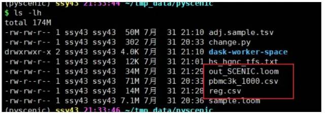
image-20230131191733555

在Linux跑完scSCENIC的流程后，接下来基于R语言，将loom数据粗处理，然后导入Seurat单细胞数据进行可视化。

Step3.sample_SCENIC.loom导入R里面进行可视化

加载R包：

##可视化
rm(list=ls())
library(Seurat)
library(SCopeLoomR)
library(AUCell)
library(SCENIC)
library(dplyr)
library(KernSmooth)
library(RColorBrewer)
library(plotly)
library(BiocParallel)
library(grid)
library(ComplexHeatmap)
library(data.table)
library(scRNAseq)
library(patchwork)
library(ggplot2) 
library(stringr)
library(circlize)

3.1 提取 out_SCENIC.loom 信息:

#### 1.提取 out_SCENIC.loom 信息
loom <- open_loom('out_SCENIC.loom') 

regulons_incidMat <- get_regulons(loom, column.attr.name="Regulons")
regulons_incidMat[1:4,1:4] 
regulons <- regulonsToGeneLists(regulons_incidMat)
regulonAUC <- get_regulons_AUC(loom,column.attr.name='RegulonsAUC')
regulonAucThresholds <- get_regulon_thresholds(loom)
tail(regulonAucThresholds[order(as.numeric(names(regulonAucThresholds)))])

embeddings <- get_embeddings(loom)  
close_loom(loom)

rownames(regulonAUC)
names(regulons)

3.2 加载SeuratData

#### 2.加载SeuratData
library(SeuratData) #加载seurat数据集  
data("pbmc3k")  
seurat.data = pbmc3k
#seurat.data = readRDS("./pbmc3k.test.seurat.Rds")
seurat.data <- seurat.data %>% NormalizeData(verbose = F) %>%
  FindVariableFeatures(selection.method = "vst", nfeatures = 2000, verbose = F) %>% 
  ScaleData(verbose = F) %>%
  RunPCA(npcs = 30, verbose = F)

n.pcs = 30
seurat.data <- seurat.data %>% 
  RunUMAP(reduction = "pca", dims = 1:n.pcs, verbose = F) %>% 
  FindNeighbors(reduction = "pca", k.param = 10, dims = 1:n.pcs)

# 这里有自带的注释
seurat.data$seurat_annotations[is.na(seurat.data$seurat_annotations)] = "B"
Idents(seurat.data) <- "seurat_annotations"
DimPlot(seurat.data,reduction = "umap",label=T )

3.3 可视化

sub_regulonAUC <- regulonAUC[,match(colnames(seurat.data),colnames(regulonAUC))]
dim(sub_regulonAUC)
seurat.data
#确认是否一致
identical(colnames(sub_regulonAUC), colnames(seurat.data))

cellClusters <- data.frame(row.names = colnames(seurat.data), 
                           seurat_clusters = as.character(seurat.data$seurat_annotations))
cellTypes <- data.frame(row.names = colnames(seurat.data), 
                        celltype = seurat.data$seurat_annotations)
head(cellTypes)
head(cellClusters)
sub_regulonAUC[1:4,1:4] 

#保存一下
save(sub_regulonAUC,cellTypes,cellClusters,seurat.data,
     file = 'for_rss_and_visual.Rdata')

B细胞有两个非常出名的转录因子，TCF4(+) 以及NR2C1(+)，接下来就可以对这两个进行简单的可视化。首先我们需要把这两个转录因子活性信息添加到降维聚类分群后的的seurat对象里面。

#B细胞有两个非常出名的转录因子，TCF4(+) 以及NR2C1(+)
regulonsToPlot = c('TCF4(+)','NR2C1(+)')
regulonsToPlot %in% row.names(sub_regulonAUC)
seurat.data@meta.data = cbind(seurat.data@meta.data ,t(assay(sub_regulonAUC[regulonsToPlot,])))

# Vis
p1 = DotPlot(seurat.data, features = unique(regulonsToPlot)) + RotatedAxis()
p2 = RidgePlot(seurat.data, features = regulonsToPlot , ncol = 2) 
p3 = VlnPlot(seurat.data, features = regulonsToPlot,pt.size = 0)
p4 = FeaturePlot(seurat.data,features = regulonsToPlot)

wrap_plots(p1,p2,p3,p4)
#可选
#scenic_res = assay(sub_regulonAUC) %>% as.matrix()
#seurat.data[["scenic"]] <- SeuratObject::CreateAssayObject(counts = scenic_res)
#seurat.data <- SeuratObject::SetAssayData(seurat.data, slot = "scale.data",
#                                  new.data = scenic_res, assay = "scenic")

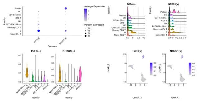
image-20230131191751021

Step4.亚群特异性转录因子分析及可视化

4.1 TF活性均值

看看不同单细胞亚群的转录因子活性平均值

### 4.1. TF活性均值
# 看看不同单细胞亚群的转录因子活性平均值
# Split the cells by cluster:
selectedResolution <- "celltype" # select resolution
cellsPerGroup <- split(rownames(cellTypes), 
                       cellTypes[,selectedResolution])

# 去除extened regulons
sub_regulonAUC <- sub_regulonAUC[onlyNonDuplicatedExtended(rownames(sub_regulonAUC)),] 
dim(sub_regulonAUC)

# Calculate average expression:
regulonActivity_byGroup <- sapply(cellsPerGroup,
                                  function(cells) 
                                    rowMeans(getAUC(sub_regulonAUC)[,cells]))

# Scale expression. 
# Scale函数是对列进行归一化，所以要把regulonActivity_byGroup转置成细胞为行，基因为列
# 参考：https://www.jianshu.com/p/115d07af3029
regulonActivity_byGroup_Scaled <- t(scale(t(regulonActivity_byGroup),
                                          center = T, scale=T)) 
# 同一个regulon在不同cluster的scale处理
dim(regulonActivity_byGroup_Scaled)
#[1] 209   9
regulonActivity_byGroup_Scaled=na.omit(regulonActivity_byGroup_Scaled)

热图查看TF分布：

Heatmap(
  regulonActivity_byGroup_Scaled,
  name                         = "z-score",
  col                          = colorRamp2(seq(from=-2,to=2,length=11),rev(brewer.pal(11, "Spectral"))),
  show_row_names               = TRUE,
  show_column_names            = TRUE,
  row_names_gp                 = gpar(fontsize = 6),
  clustering_method_rows = "ward.D2",
  clustering_method_columns = "ward.D2",
  row_title_rot                = 0,
  cluster_rows                 = TRUE,
  cluster_row_slices           = FALSE,
  cluster_columns              = FALSE)

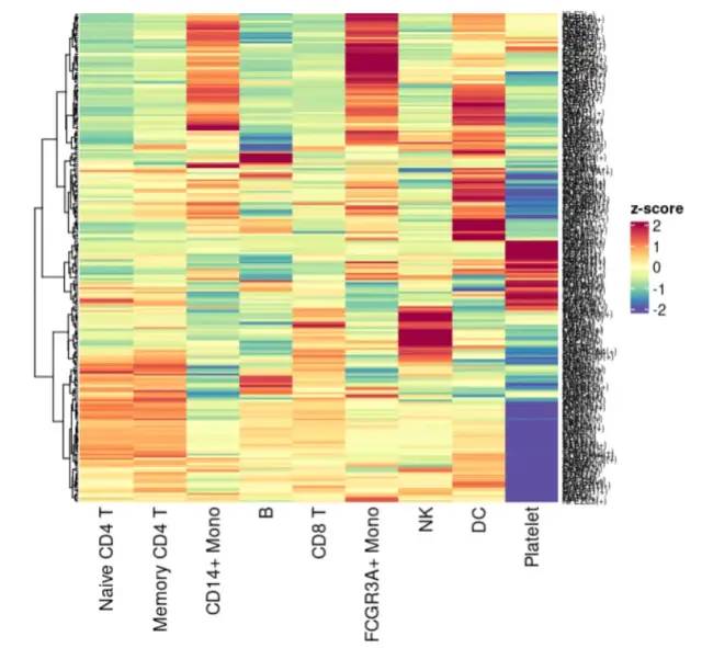
image-20230131191806586

可以看到，确实每个单细胞亚群都是有自己的特异性的激活的转录因子。

4.2 rss查看特异TF

不过，SCENIC包自己提供了一个 calcRSS函数，帮助我们来挑选各个单细胞亚群特异性的转录因子，全称是：Calculates the regulon specificity score

参考文章：The RSS was first used by Suo et al. in: Revealing the Critical Regulators of Cell Identity in the Mouse Cell Atlas. Cell Reports (2018). doi: 10.1016/j.celrep.2018.10.045 运行超级简单。

### 4.2. rss查看特异TF
rss <- calcRSS(AUC=getAUC(sub_regulonAUC), 
               cellAnnotation=cellTypes[colnames(sub_regulonAUC), selectedResolution]) 
rss=na.omit(rss) 
rssPlot <- plotRSS(rss)
plotly::ggplotly(rssPlot$plot)

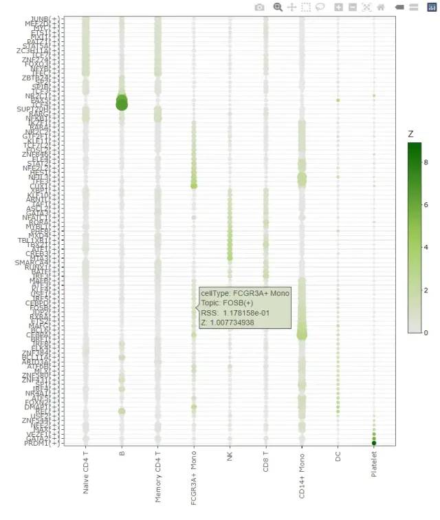
image-20220731224415686

4.3 其他查看TF方式

rss=regulonActivity_byGroup_Scaled
head(rss)
df = do.call(rbind,
             lapply(1:ncol(rss), function(i){
               dat= data.frame(
                 path  = rownames(rss),
                 cluster =   colnames(rss)[i],
                 sd.1 = rss[,i],
                 sd.2 = apply(rss[,-i], 1, median)  
               )
             }))
df$fc = df$sd.1 - df$sd.2
top5 <- df %>% group_by(cluster) %>% top_n(5, fc)
rowcn = data.frame(path = top5$cluster) 
n = rss[top5$path,] 
#rownames(rowcn) = rownames(n)
pheatmap(n,
         annotation_row = rowcn,
         show_rownames = T)

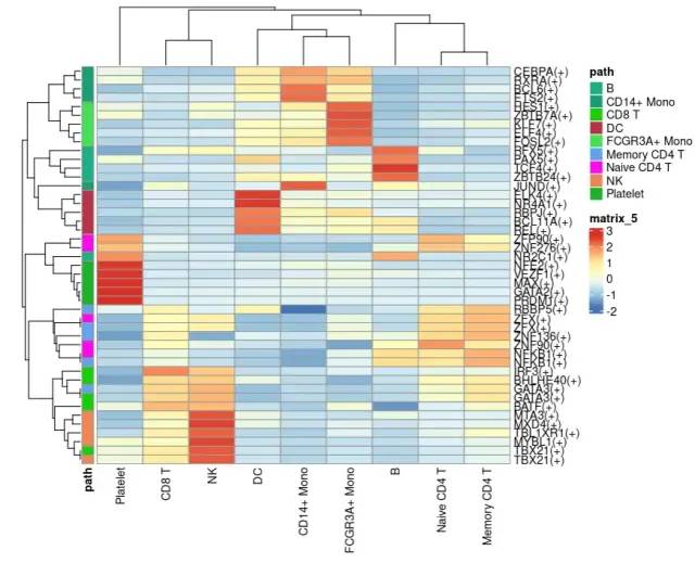
image-20230131191851169- END -

本文参与腾讯云自媒体分享计划，分享自微信公众号。

原始发表：2023-01-31，如有侵权请联系 cloudcommunity@tencent.com 删除

数据库

sql

python

本文分享自生信技能树微信公众号，前往查看

如有侵权，请联系 cloudcommunity@tencent.com 删除。

本文参与腾讯云自媒体分享计划，欢迎热爱写作的你一起参与！

数据库

sql

python

登录后参与评论

0 条评论

热度