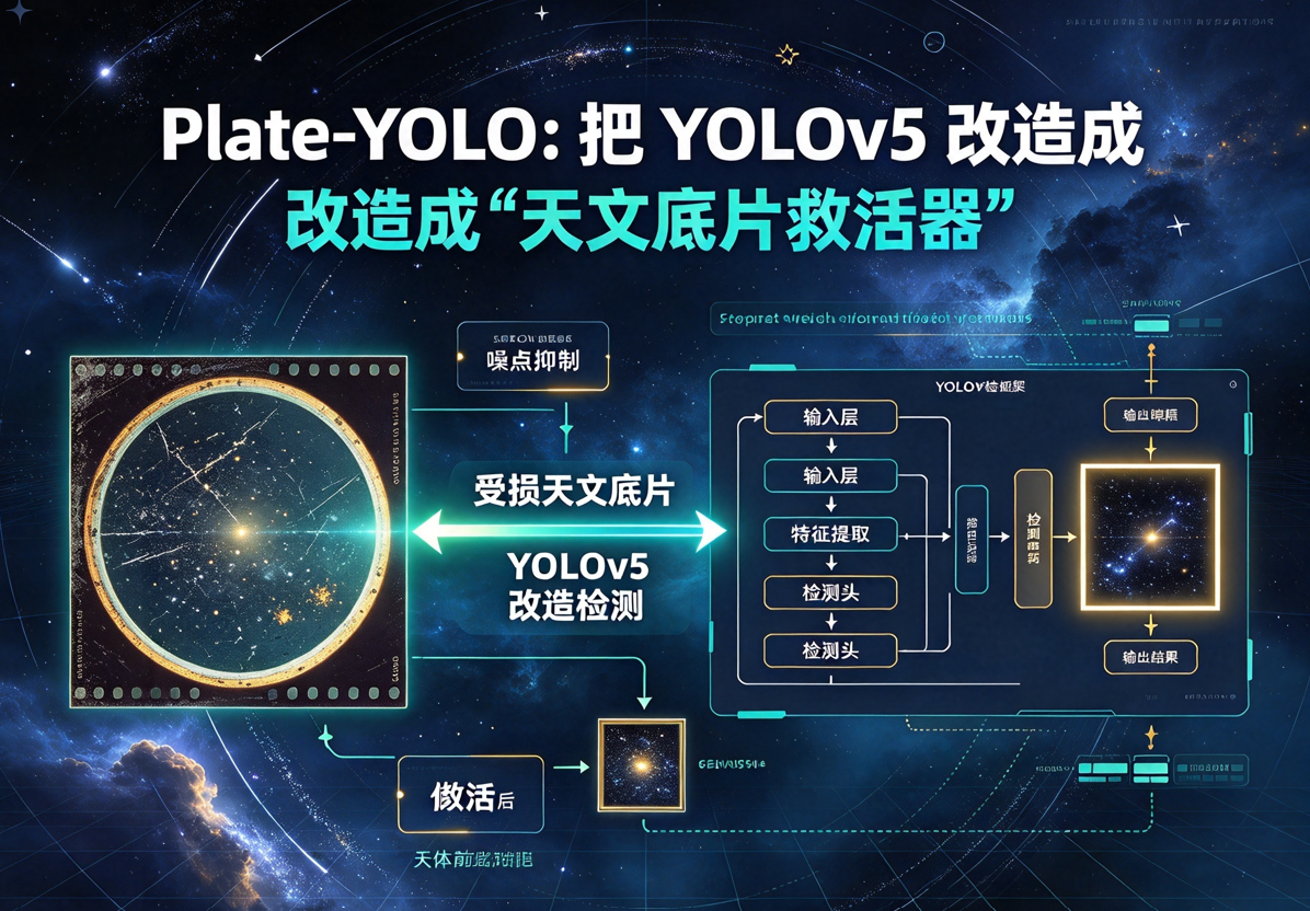
Plate-YOLO:把 YOLOv5 改造成"天文底片救活器"
原创
Plate-YOLO:把 YOLOv5 改造成"天文底片救活器"
原创
AI小怪兽
发布于 2026-11-03 13:23:02
发布于 2026-11-03 13:23:02
Plate-YOLO:把 YOLOv5 改造成"天文底片救活器"
上海天文台团队(arXiv:2610.25677)把"源检测 + 恒星分类"塞进一个检测器,输出星表直接喂给天体测量求解器,专治历史玻璃底片因划痕、霉斑、乳胶退化导致的解算失败。150 张传统流程解不开的失败底片,救回了 146 张。
博主简介

AI小怪兽 | 计算机视觉布道者 | 视觉检测领域创新者

深耕计算机视觉与深度学习领域,专注于目标检测前沿技术的探索与突破。长期致力于YOLO系列算法的结构性创新、性能极限优化与工业级落地实践,旨在打通从学术研究到产业应用的最后一公里。
🚀 核心专长与技术创新
- YOLO算法结构性创新:于CSDN平台原创发布《YOLO26魔术师》、《YOLO11魔术师》等全系列深度专栏。系统性提出并开源了多项原创自研模块,在模型轻量化设计、多维度注意力机制融合、特征金字塔重构等关键方向完成了一系列突破性实践,为行业提供了具备高参考价值的技术路径与完整解决方案。
- 技术生态建设与知识传播:独立运营 “计算机视觉大作战” 公众号(粉丝2.3万),成功构建高质量的技术交流社群。致力于将复杂算法转化为通俗易懂的解读与可复现的工程代码,显著降低了计算机视觉的技术入门门槛。
🏆 行业影响力与商业实践
- 荣获腾讯云年度影响力作者与创作之星奖项,内容质量与专业性获行业权威平台认证。
- 全网累计拥有 8万+ 垂直领域技术受众,专栏文章总阅读量突破百万,在目标检测领域形成了广泛的学术与工业影响力。
- 具备丰富的企业级项目交付经验,曾为工业视觉检测、智慧城市安防等多个关键领域提供定制化的算法模型与解决方案,驱动业务智能化升级。
💡 未来方向与使命
秉持 “让每一行代码都有温度” 的技术理念,未来将持续聚焦于实时检测、语义分割及工业缺陷检测的商业化闭环等核心方向。愿与业界同仁协同创新,共同推动技术边界,以坚实的技术能力赋能实体经济与行业变革。
一、摘要
历史天文照相底片是"动态宇宙"独一无二的百年长基线记录,但退化与结构噪声常常让自动化天体测量配准(astrometric calibration)直接卡死。论文提出 Plate-YOLO:用一个检测器同时完成源检测与恒星分类,再把星表送给独立的天体测量求解器。检测器在 YOLOv5 基础上做了四处针对性改造——Space-to-Depth(SPD)特征重排、SimAM 注意力、高分辨率 P2 检测头、面向小框的归一化 Wasserstein 距离损失(NWD Loss);并用 Gaia 引导的微调把已解算底片变成新档案的标签。
一句话结论:在 150 张传统流水线彻底失败的底片上,中国训练的模型先救回 40 张,再做目标档案微调又救回 106 张,整体恢复率 146/150 = 97.3%;源检测耗时 6.61 秒对 16.73 秒,提速约 2.53 倍。
伪代码如下:
# plate_yolo_pseudocode.py
# -*- coding: utf-8 -*-
"""
Plate-YOLO 伪代码实现
参考论文: Plate-YOLO: An End-to-End Object Detection Framework for
         Robust Astrometric Registration of Historical Plates
         (arXiv:2610.25677)

说明:本文件为算法逻辑伪代码,用于理解论文方法流程,
     并非可直接运行的完整实现。部分组件(如骨干网络、PANet、
     检测头内部细节)以高层接口表示,重点展示论文的创新模块与训练策略。
"""

import torch
import torch.nn as nn
import torch.nn.functional as F
import math


# ============================================================
# 1. 基础模块
# ============================================================

class SpaceToDepth(nn.Module):
    """
    Space-to-Depth (SPD) 模块[reference:0]
    将 (H, W, C) 特征图通过 2×2 空间邻域重排为 (H/2, W/2, 4C),
    在降低空间分辨率的同时保留像素级细粒度线索。
    """
    def __init__(self, block_size=2):
        super().__init__()
        self.block_size = block_size

    def forward(self, x):
        # x: (B, C, H, W)
        B, C, H, W = x.shape
        s = self.block_size
        # 将空间维度按 s×s 划分并重排到通道维度
        x = x.view(B, C, H // s, s, W // s, s)
        x = x.permute(0, 1, 3, 5, 2, 4).contiguous()
        x = x.view(B, C * s * s, H // s, W // s)
        return x


class SimAM(nn.Module):
    """
    Simple Parameter-Free Attention Module (SimAM)[reference:1]
    基于能量函数的 3D 注意力,无额外可学习参数,
    对特征激活进行重加权,以抑制结构化背景噪声。
    """
    def __init__(self, e_lambda=1e-4):
        super().__init__()
        self.e_lambda = e_lambda

    def forward(self, x):
        # x: (B, C, H, W)
        n = x.shape[2] * x.shape[3] - 1
        d = (x - x.mean(dim=[2, 3], keepdim=True)).pow(2)
        v = d.sum(dim=[2, 3], keepdim=True) / n
        # 能量函数:E = 1 / (v + λ)
        e_inv = d / (4 * (v + self.e_lambda)) + 0.5
        return x * torch.sigmoid(e_inv)


# ============================================================
# 2. Plate-YOLO 主干与特征融合(高层表示)
# ============================================================

class CSPNetBackboneWithSPD(nn.Module):
    """
    在 CSPNet 浅层嵌入 SPD 模块的骨干网络[reference:2]
    """
    def __init__(self):
        super().__init__()
        # 伪代码:实际实现中由多个 CBS / C3 块组成
        self.stem = nn.Sequential(
            nn.Conv2d(1, 32, 3, 1, 1),   # 灰度历史底片
            nn.BatchNorm2d(32),
            nn.SiLU()
        )
        self.spd = SpaceToDepth(block_size=2)
        # ... 后续 CSP 块(省略)
        self.csp_layers = nn.Identity()  # 占位

    def forward(self, x):
        x = self.stem(x)
        x = self.spd(x)          # 浅层引入 SPD,保留细小源信号
        x = self.csp_layers(x)
        return x


class PANetNeckWithSimAM(nn.Module):
    """
    PANet 多尺度融合颈部,在融合节点插入 SimAM[reference:3]
    """
    def __init__(self, in_channels_list=(64, 128, 256, 512)):
        super().__init__()
        # 伪代码:实际实现包含上采样、下采样与 C3 融合块
        self.simam_p2 = SimAM()
        self.simam_p3 = SimAM()
        self.simam_p4 = SimAM()
        self.simam_p5 = SimAM()
        # ... 融合卷积(省略)

    def forward(self, features):
        # features: 来自骨干的多尺度特征 [P2, P3, P4, P5]
        p2, p3, p4, p5 = features
        # 在融合节点施加 SimAM 注意力
        p2 = self.simam_p2(p2)
        p3 = self.simam_p3(p3)
        p4 = self.simam_p4(p4)
        p5 = self.simam_p5(p5)
        # ... 上采样与融合(省略)
        return [p2, p3, p4, p5]


class P2DetectionHead(nn.Module):
    """
    微尺度高分辨率检测头(P2)[reference:4]
    在标准 P3-P5 基础上增加 P2 头,提升对仅占数像素的天体源的定位灵敏度。
    """
    def __init__(self, num_classes=2, num_anchors=3):
        super().__init__()
        # 每个位置预测: tx, ty, tw, th, obj, cls
        self.conv = nn.Conv2d(64, num_anchors * (5 + num_classes), 1)

    def forward(self, feature_map):
        return self.conv(feature_map)


# ============================================================
# 3. 联合损失函数(核心)[reference:5]
# ============================================================

def normalized_wasserstein_distance_loss(pred_boxes, gt_boxes, C=12.8):
    """
    Normalized Wasserstein Distance (NWD) 回归损失[reference:6]
    将边界框建模为二维高斯分布,对微小框和非重叠框仍提供有效梯度。

    参数:
        pred_boxes: (N, 4)  [xc, yc, w, h]
        gt_boxes:   (N, 4)
        C:          归一化常数,论文取 12.8
    返回:
        loss: 标量
    """
    # 1. 构造高斯均值与对角协方差
    mu_p = pred_boxes[:, :2]                     # (N, 2)
    mu_g = gt_boxes[:, :2]
    sigma_p = torch.diag_embed(pred_boxes[:, 2:] ** 2 / 4)  # (N, 2, 2)
    sigma_g = torch.diag_embed(gt_boxes[:, 2:] ** 2 / 4)

    # 2. 二阶 Wasserstein 距离的平方
    # W2^2 = ||μp − μg||^2 + Tr(Σp + Σg − 2(Σp^{1/2} Σg Σp^{1/2})^{1/2})
    # 对于对角协方差,简化为:
    # W2^2 = ||μp − μg||^2 + (wp−wg)^2/4 + (hp−hg)^2/4
    mu_diff_sq = ((mu_p - mu_g) ** 2).sum(dim=1)               # (N,)
    wh_diff_sq = ((pred_boxes[:, 2:] - gt_boxes[:, 2:]) ** 2).sum(dim=1) / 4
    W2_sq = mu_diff_sq + wh_diff_sq

    # 3. 归一化 NWD 损失
    nwd = torch.exp(-torch.sqrt(W2_sq + 1e-7) / C)
    loss = 1.0 - nwd
    return loss.mean()


def objectness_loss(pred_obj, target, alpha=0.25, gamma=2.0, level_weights=None):
    """
    动态缩放 Focal Loss 计算目标性损失[reference:7]
    对不同检测头层级(P2/P3/P4/P5)施加不同权重,最高权重赋予 P2 头。
    """
    # pred_obj:   (N,)
    # target:     (N,)  0/1
    p = torch.sigmoid(pred_obj)
    pt = torch.where(target == 1, p, 1 - p)
    alpha_t = torch.where(target == 1, alpha, 1 - alpha)
    focal = -alpha_t * (1 - pt) ** gamma * torch.log(pt + 1e-7)

    # 按层级加权(伪代码:假设传入的 level_weights 已按样本分组)
    if level_weights is not None:
        focal = focal * level_weights
    return focal.mean()


def classification_loss(pred_cls, target_cls):
    """
    恒星/伪源二分类损失(BCE)[reference:8]
    """
    return F.binary_cross_entropy_with_logits(pred_cls, target_cls.float())


def plate_yolo_total_loss(preds, targets, lambda_box=0.05, lambda_obj=1.0, lambda_cls=0.5):
    """
    联合损失 L_total = λ_box * L_box_NWD + λ_obj * L_obj + λ_cls * L_cls[reference:9]
    """
    # 伪代码:preds 为包含各尺度预测的字典
    box_loss = normalized_wasserstein_distance_loss(
        preds["boxes"], targets["boxes"]
    )
    obj_loss = objectness_loss(
        preds["objectness"], targets["objectness"], level_weights=preds.get("level_weights")
    )
    cls_loss = classification_loss(
        preds["class_logits"], targets["class_labels"]
    )
    total = lambda_box * box_loss + lambda_obj * obj_loss + lambda_cls * cls_loss
    return total, {"box_nwd": box_loss, "obj": obj_loss, "cls": cls_loss}


# ============================================================
# 4. 完整 Plate-YOLO 前向传播(推理流程)
# ============================================================

class PlateYOLO(nn.Module):
    """
    Plate-YOLO 整体模型[reference:10]
    """
    def __init__(self, num_classes=2):
        super().__init__()
        self.backbone = CSPNetBackboneWithSPD()
        self.neck = PANetNeckWithSimAM()
        # 四个检测头:P2(微尺度)、P3、P4、P5
        self.head_p2 = P2DetectionHead(num_classes)
        self.head_p3 = P2DetectionHead(num_classes)
        self.head_p4 = P2DetectionHead(num_classes)
        self.head_p5 = P2DetectionHead(num_classes)

    def forward(self, x):
        """
        x: 灰度历史底片切块,形状 (B, 1, H, W)
        返回: 多尺度检测结果
        """
        features = self.backbone(x)                    # 多尺度特征
        p2, p3, p4, p5 = self.neck(features)           # PANet + SimAM
        out_p2 = self.head_p2(p2)
        out_p3 = self.head_p3(p3)
        out_p4 = self.head_p4(p4)
        out_p5 = self.head_p5(p5)
        return [out_p2, out_p3, out_p4, out_p5]

    @torch.no_grad()
    def inference(self, x, conf_thresh=0.5, nms_iou=0.2):
        """
        推理阶段后处理[reference:11]:
        置信度过滤 + 按类别全局 NMS + 坐标还原
        """
        raw_outputs = self.forward(x)
        # 伪代码:解码边界框、置信度、类别概率
        boxes, scores, labels = decode_predictions(raw_outputs)
        # 置信度阈值
        mask = scores >= conf_thresh
        boxes, scores, labels = boxes[mask], scores[mask], labels[mask]
        # 按类别全局 NMS(IoU 阈值 0.2)
        keep = class_wise_nms(boxes, scores, labels, iou_thresh=nms_iou)
        return boxes[keep], scores[keep], labels[keep]


def decode_predictions(raw_outputs):
    """占位:将检测头原始输出解码为边界框、置信度、类别"""
    raise NotImplementedError


def class_wise_nms(boxes, scores, labels, iou_thresh=0.2):
    """占位:按类别执行非极大值抑制"""
    raise NotImplementedError


# ============================================================
# 5. 跨档案 Gaia 引导微调[reference:12]
# ============================================================

def gaia_guided_finetune(model, Ds_loader, Dt_loader, theta_s, num_epochs=50,
                         lambda_t=1.0, lambda_reg=0.01, lr=1e-4):
    """
    Gaia-guided Fine-tuning[reference:13]

    参数:
        model:        预训练的 Plate-YOLO 模型(源域 Base Model)
        Ds_loader:    源域数据加载器(带标签)
        Dt_loader:    目标域数据加载器(Gaia 交叉匹配自动生成的标签)
        theta_s:      冻结的源域模型权重(用于正则化)
        lambda_t:     目标域损失权重
        lambda_reg:   权重偏离正则化系数
    """
    optimizer = torch.optim.Adam(model.parameters(), lr=lr)
    theta_s = {k: v.clone().detach() for k, v in theta_s.items()}

    for epoch in range(num_epochs):
        model.train()
        for batch_s, batch_t in zip(Ds_loader, Dt_loader):
            # 1. 源域损失
            preds_s = model(batch_s["image"])
            L_det_s, _ = plate_yolo_total_loss(preds_s, batch_s["target"])

            # 2. 目标域损失(Gaia 引导标签)
            preds_t = model(batch_t["image"])
            L_det_t, _ = plate_yolo_total_loss(preds_t, batch_t["target"])

            # 3. 正则化项:惩罚偏离源域权重的程度
            reg_loss = 0.0
            for name, param in model.named_parameters():
                if name in theta_s:
                    reg_loss = reg_loss + ((param - theta_s[name]) ** 2).sum()

            # 4. 总损失 Eq.(7)
            loss = L_det_s + lambda_t * L_det_t + lambda_reg * reg_loss

            optimizer.zero_grad()
            loss.backward()
            optimizer.step()

        print(f"[Finetune] Epoch {epoch + 1}/{num_epochs} | loss = {loss.item():.4f}")

    return model


# ============================================================
# 6. 仪器亮度估计与源排序[reference:14]
# ============================================================

def estimate_instrumental_magnitude(fits_image, bbox, mag_zero_point=0.0):
    """
    从原始未拉伸 FITS 图像估计仪器星等,用于源排序(非定标光度)[reference:15]

    参数:
        fits_image: 原始像素数组 (H, W)
        bbox:       [xmin, ymin, xmax, ymax]
        mag_zero_point: 加性常数,不影响底片内排序
    返回:
        m_inst: 仪器星等(越小越亮);若背景扣除后非正则返回 +inf
    """
    xmin, ymin, xmax, ymax = bbox
    # 1. 几何中心作为孔径中心
    xc = (xmin + xmax) / 2.0
    yc = (ymin + ymax) / 2.0
    w = xmax - xmin
    h = ymax - ymin

    # 2. 椭圆测量孔径:半轴 (a, b) = 0.75 × (w, h)
    a = 0.75 * w
    b = 0.75 * h

    # 3. 局部背景:同心椭圆环带 [1.25×(w,h), 1.75×(w,h)] 的中位数
    a_in, b_in = 1.25 * w, 1.25 * h
    a_out, b_out = 1.75 * w, 1.75 * h
    background_pixels = extract_annulus_pixels(fits_image, xc, yc, a_in, b_in, a_out, b_out)
    B = torch.median(background_pixels) if len(background_pixels) > 0 else 0.0

    # 4. 背景扣除后的像元值和 F(在原始未拉伸图像上计算)
    aperture_pixels = extract_elliptical_pixels(fits_image, xc, yc, a, b)
    F = (aperture_pixels - B).sum()

    # 5. 仪器星等
    if F > 0:
        return -2.5 * math.log10(F.item()) + mag_zero_point
    else:
        return float("inf")  # 最低排序


def extract_elliptical_pixels(image, xc, yc, a, b):
    """占位:提取椭圆内像素值"""
    raise NotImplementedError


def extract_annulus_pixels(image, xc, yc, a_in, b_in, a_out, b_out):
    """占位:提取椭圆环带内像素值"""
    raise NotImplementedError


def rank_and_select_sources(detections, fits_image, max_sources=500):
    """
    按仪器星等排序,选取前 max_sources 个源送入 Astrometry.net[reference:16]

    参数:
        detections: 列表,每个元素包含 bbox 和 class_label(仅保留 stellar)
        fits_image: 原始未拉伸 FITS 像素数组
    返回:
        selected: 按亮度排序的源列表(最多 max_sources 个)
    """
    stellar_dets = [d for d in detections if d["class_label"] == 1]  # 1 = stellar
    scored = []
    for det in stellar_dets:
        m_inst = estimate_instrumental_magnitude(fits_image, det["bbox"])
        scored.append((m_inst, det))

    # 按仪器星等升序(越亮越靠前)
    scored.sort(key=lambda x: x[0])
    selected = [det for _, det in scored[:max_sources]]
    return selected


# ============================================================
# 7. 全底片推理与天体测量求解流水线(伪代码)
# ============================================================

def full_plate_pipeline(model, plate_image, patch_size=256, stride=230,
                        conf_thresh=0.5, nms_iou=0.2, max_sources=500):
    """
    全底片推理流程[reference:17][reference:18]

    步骤:
        1. 将大底片切分为 256×256 切块,步长 230,边缘对齐;
        2. Plate-YOLO 逐块推理,保留 stellar 类别且置信度 ≥ 0.5;
        3. 将局部框坐标映射回全底片坐标;
        4. 全局按类别 NMS(IoU=0.2)去重;
        5. 从原始未拉伸 FITS 图像估计仪器星等并排序;
        6. 取前 500 个源送入 Astrometry.net。
    """
    H, W = plate_image.shape
    all_dets = []

    # 1. 切块推理
    for y in range(0, H, stride):
        for x in range(0, W, stride):
            y0, y1 = y, min(y + patch_size, H)
            x0, x1 = x, min(x + patch_size, W)
            patch = plate_image[y0:y1, x0:x1]
            patch_tensor = preprocess_patch(patch)
            boxes, scores, labels = model.inference(patch_tensor, conf_thresh, nms_iou)
            # 2. 坐标映射回全底片
            for bbox, score, label in zip(boxes, scores, labels):
                if label == 1:  # stellar
                    global_bbox = [
                        bbox[0] + x0, bbox[1] + y0,
                        bbox[2] + x0, bbox[3] + y0
                    ]
                    all_dets.append({"bbox": global_bbox, "score": score, "class_label": label})

    # 3. 全局 NMS(按类别)
    all_dets = global_nms(all_dets, iou_thresh=nms_iou)

    # 4. 仪器亮度排序并选取前 max_sources
    selected = rank_and_select_sources(all_dets, plate_image, max_sources)

    # 5. 送入 Astrometry.net(伪代码)
    source_catalog = [{"x": (d["bbox"][0] + d["bbox"][2]) / 2,
                       "y": (d["bbox"][1] + d["bbox"][3]) / 2}
                      for d in selected]
    wcs_solution = astrometry_net_solve(source_catalog)
    return wcs_solution


def preprocess_patch(patch):
    """占位:归一化、转张量"""
    raise NotImplementedError


def global_nms(detections, iou_thresh=0.2):
    """占位:全局 NMS"""
    raise NotImplementedError


def astrometry_net_solve(source_catalog):
    """占位:调用 Astrometry.net 求解 WCS"""
    raise NotImplementedError


# ============================================================
# 主流程示意
# ============================================================
if __name__ == "__main__":
    print("Plate-YOLO 伪代码流程:")
    print("1. 构建 PlateYOLO 模型(SPD + SimAM + P2 头)")
    print("2. 在源域数据上预训练,优化联合损失 L_total")
    print("3. 对目标域零样本推理,保留成功求解的底片")
    print("4. 利用 Gaia 交叉匹配自动生成目标域标签 D_t")
    print("5. 联合 D_s 和 D_t 微调,损失含权重正则化项")
    print("6. 全底片切块推理 → 全局 NMS → 仪器亮度排序 → 前 500 源送入 Astrometry.net")
二、研究背景和意义
历史天文底片的价值在于"时间"。Harvard DASCH 数字化约 45 万张、APPLAUSE 整合 7 万张、SuperCOSMOS 覆盖南天施密特底片,上海天文台也用自研高精度扫描仪集中数字化了约 3 万张中国底片。但要让这些档案发挥科学价值,第一步就是精确的天体测量配准。

传统配准流水线 Figure 1
传统流水线(Figure 1)是一套串行范式:全幅源检测(常用 SExtractor 阈值算法)→ 恒星分类 → 盲解算(Astrometry.net)→ 用 Gaia 等精确星表做 WCS 精解。问题出在最前端的源检测:底片长期保存会退化出划痕、霉斑、乳胶缺陷和复杂结构噪声,阈值类算法在这种退化数据上大量漏检、误检,直接拖垮后续配准。
这正是"在退化前补局部证据"的范式问题——和满场小目标、噪点画质的检测场景同源。
三、创新点
Plate-YOLO 对 YOLOv5 做了四处改造,专攻"微尺度恒星点源 + 退化底片":
- Space-to-Depth(SPD)特征重排:用 SPD 下采样替代 stride-2 卷积,避免小目标特征在下采样时丢损。
- SimAM 注意力:无参注意力机制,增强退化区域的特征响应。
- 高分辨率 P2 检测头(Micro-Scale Head):新增 P2 层,专门抓微尺度恒星点源。
- NWD Loss:用归一化 Wasserstein 距离度量小框相似度,比 IoU 类损失对小目标更鲁棒。
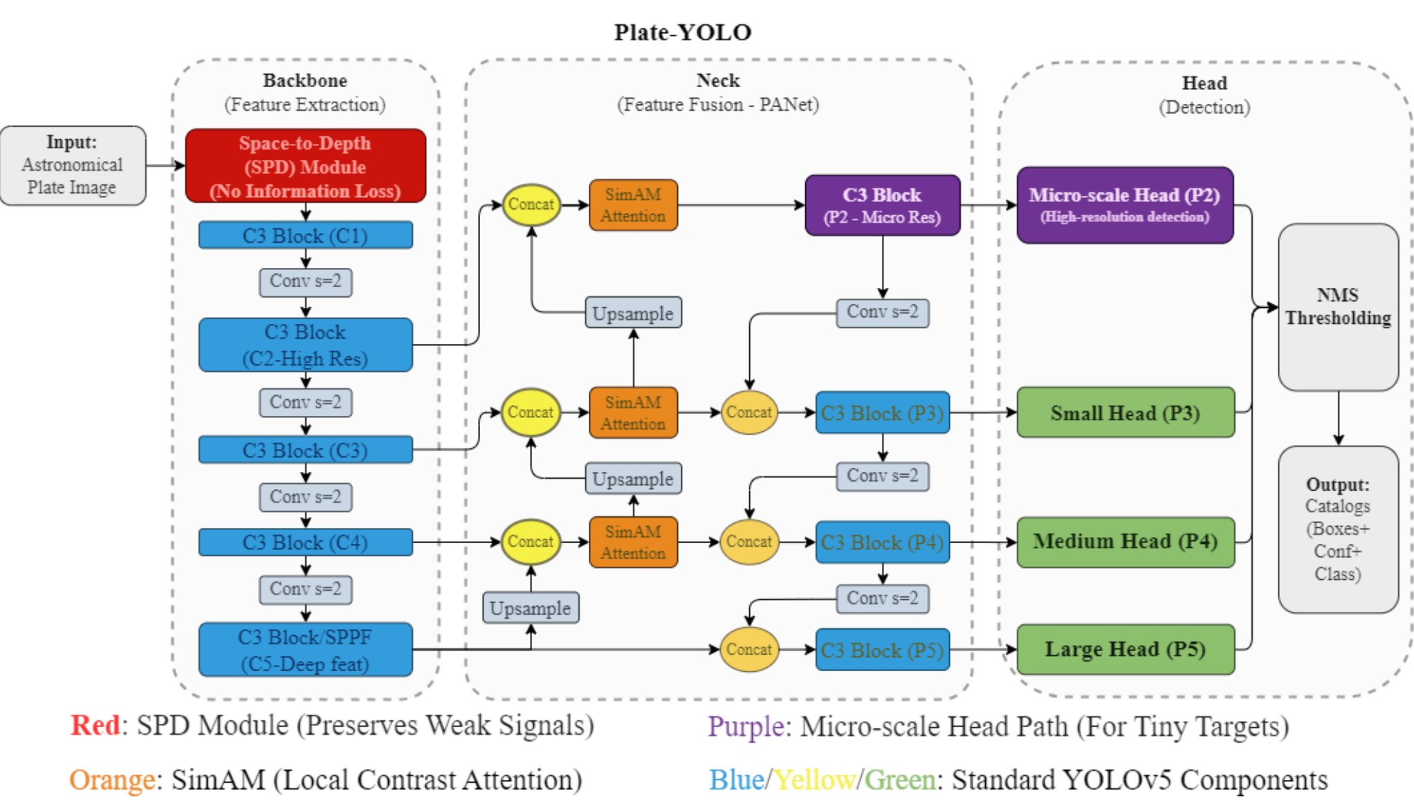
Plate-YOLO 架构 Figure 2
配套工程也不少:重叠滑动窗口切分 + asinh 映射处理单色底片的大动态范围;Gaia 引导微调用已解算底片构造标签,再迁移到新档案;输出星表(边界框 + 置信度 + 类别),置信度阈值过滤背景。
消融实验(Table 3)把每个模块的贡献拆得清清楚楚:
模型变体 | 新增组件 | Precision(%) | Recall(%) | AP@0.5 |
|---|---|---|---|---|
Baseline(YOLOv5) | None | 85.6 | 78.4 | 0.754 |
Variant 1 | + NWD Loss | 91.8 | 82.3 | 0.803 |
Variant 2 | + SPD Module | 92.4 | 85.1 | 0.826 |
Variant 3 | + SimAM | 95.5 | 84.8 | 0.841 |
Plate-YOLO | + P2 Head | 97.0 | 88.0 | 0.874 |
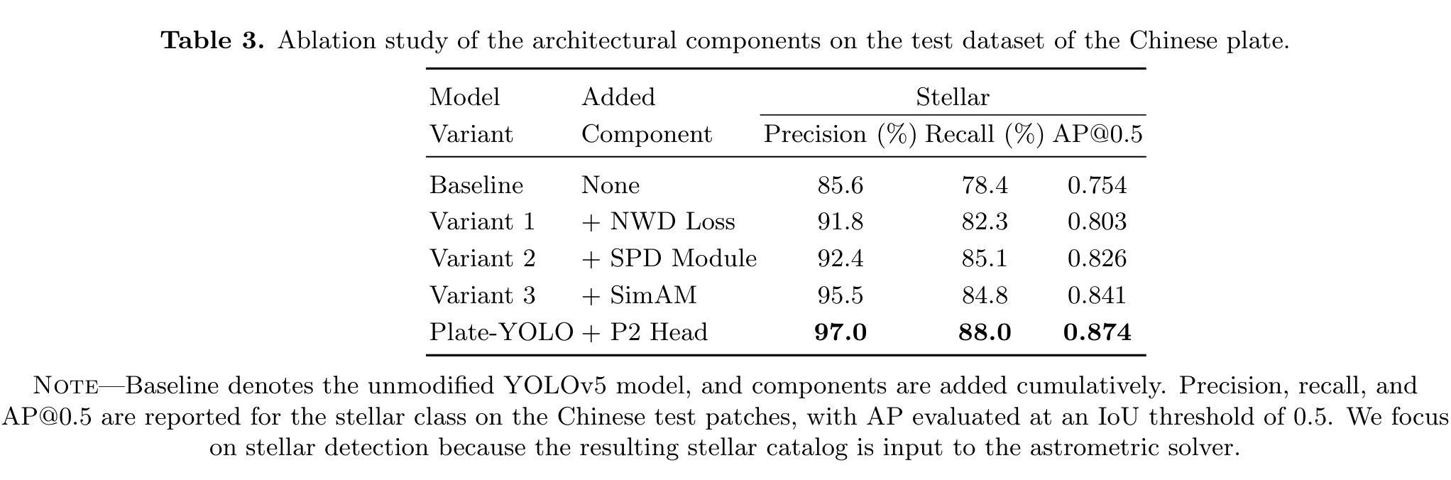
消融实验 Table 3
每个模块都稳稳涨点,最后一把 P2 头把召回率从 84.8% 拉到 88.0%,AP@0.5 累计提升 0.754 → 0.874。
数据集(Table 1,Chinese archive)按 Train/Val/Test 切分,含整片、切图、恒星与伪源统计:
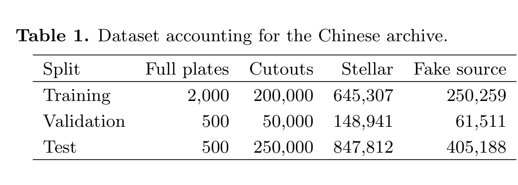
数据集 Table 1
四、创新点解读(非论文原文,纯属个人观点)
以下解读为个人工程视角,不代表论文作者立场。
为什么是"微尺度"? 恒星在底片上就是点源(PSF 尺度),比自然场景目标小一两个数量级,常规 YOLO 的 P5 大目标头根本抓不到。P2 头在高分辨率特征上做检测,等于给网络配了一副"放大镜"。
SPD 的本质:普通 stride-2 卷积下采样会跳着取像素、丢掉高频细节;SPD 把空间维度重排到通道维度,等效"无损下采样"。对细密恒星点阵这种高频纹理,差别立竿见影。
NWD 为什么对小框友好:小框稍一错位,IoU 就跌到 0,梯度消失;Wasserstein 距离度量的是两框"分布"的相似度,对微小偏移平滑鲁棒,回归更稳定。
落到 YOLO 工程线(结合本人 YOLO11/26 实践):这套"退化数据 + 小目标"的组合拳——SPD 补特征、SimAM 提响应、P2 抓微尺度、NWD 稳回归——对 YOLO11/26 同样可迁移。浙BA 满场小目标、退化画质的检测场景,与老底片的退化点源同源:在特征退化前补局部证据。论文验证的是天文档案,思路可平移到体育场景的稳健检测。
五、实验结果
恢复率(核心):150 张传统流水线彻底失败的底片,中国训练模型先救回 40 张,Gaia 引导微调再救回 106 张,合计 146/150 = 97.3%。仅 4 张彗星目标底片在微调后仍无解(见第六节)。
检测性能(Figure 4,106 张新恢复底片):微调模型的完备率峰值约 95%(基线约 65%),在亮度排序范围内保持 60% 以上;目录纯度也优于基线与 SExtractor 传统流水线。
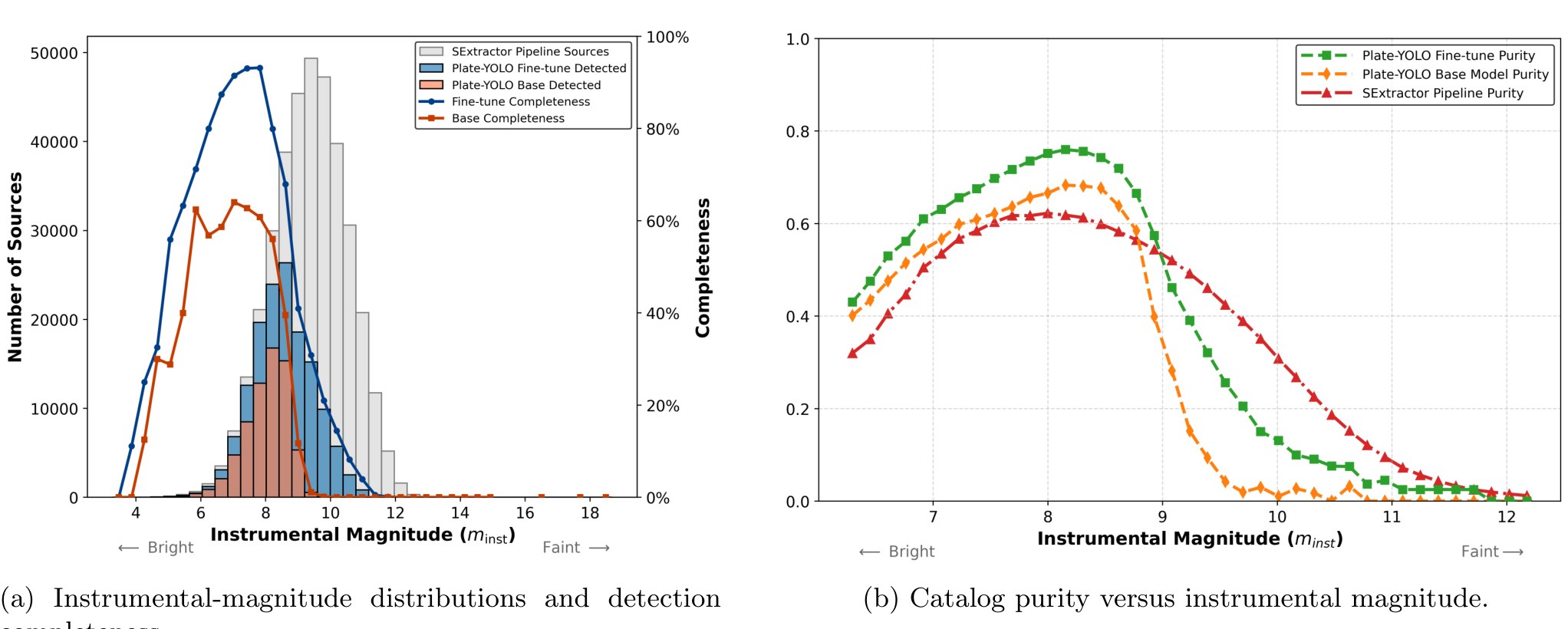
检测性能 Figure 4
位置精度(Figure 5/6):106 张新恢复底片中位 plate-level RMS = 0.563",径向残差 0.42–0.44" 且无明显向外递增;在 500 张已解算底片上,Plate-YOLO 对 308 张(61.6%) RMS 更小,配对中位差 -0.022"。
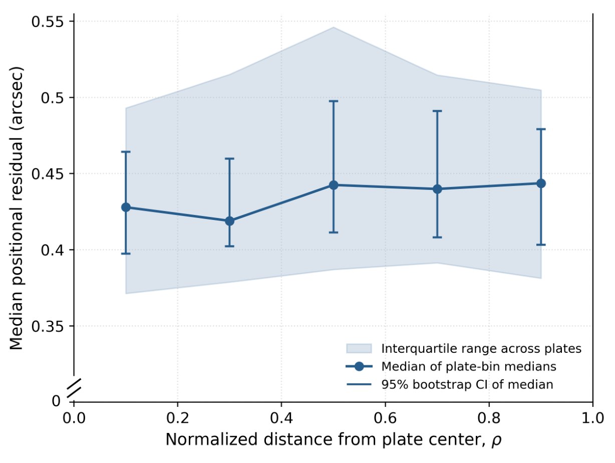
径向残差 Figure 5
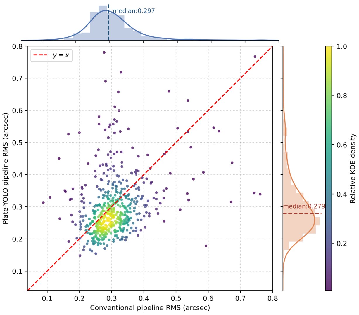
RMS 对比 Figure 6
速度(Table 2):检测阶段 Plate-YOLO 6.61 秒 vs SExtractor 16.73 秒,2.53 倍;含配准全流程 7.40 秒 vs 19.36 秒,2.62 倍。更干净星表还把 Astrometry.net 解算时间从 2.63 秒压到 0.79 秒。
方法 | 硬件 | 源提取(s) | 配准(s) | 总计(s) |
|---|---|---|---|---|
Plate-YOLO | RTX 3090(GPU) | 6.61 | 0.79 | 7.40 |
SExtractor | i9-10900(CPU) | 16.73 | 2.63 | 19.36 |

速度对比 Table 2
六、展望
论文坦承,当前性能仍依赖可用参考星表、训练标签构造方式和所考察的底片群体,需要在更多仪器与档案上进一步验证。4 张含彗星的退化底片至今无解——彗星占据视场大片面积、拖尾污染背景,恰好暴露了点源假设的边界。
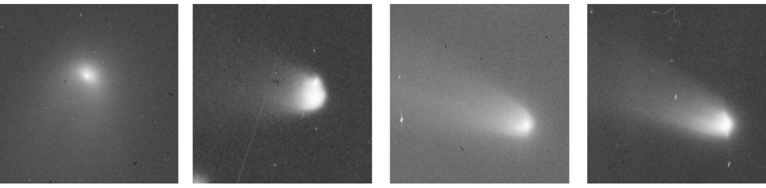
失败案例 Figure 3
(非论文原文,纯属个人观点)对 YOLO 工程线而言,Plate-YOLO 给出了一条清晰的"档案特异性适配"路径:同一套检测骨架,靠 SPD + SimAM + P2 + NWD 四件套适配退化数据。值得在 YOLO11/26 上复现这组组合,验证它对满场小目标、噪点画质场景的迁移增益。
原创声明:本文系作者授权腾讯云开发者社区发表,未经许可,不得转载。
如有侵权,请联系 cloudcommunity@tencent.com 删除。
目录
腾讯云开发者

Copyright © 2013 - 2026 Tencent Cloud. All Rights Reserved. 腾讯云 版权所有
深圳市腾讯计算机系统有限公司 ICP备案/许可证号:粤B2-20090059  粤公网安备44030502008569号
腾讯云计算(北京)有限责任公司 京ICP证150476号 | 京ICP备11018762号