比monocle更快的slingshot-CNS高分文章常用

比monocle更快的slingshot-CNS高分文章常用

生信菜鸟团
发布于 2023-09-09 17:12:24
发布于 2023-09-09 17:12:24
单细胞一文全打通
slingshot包可以对单细胞RNA-seq数据进行细胞分化谱系构建和伪时间推断,它利用细胞聚类簇和空间降维信息,以无监督或半监督的方式学习细胞聚类群之间的关系,揭示细胞聚类簇之间的全局结构,并将该结构转换为由一维变量表示的平滑谱系,称之为“伪时间”。
运行slingshot的至少需要两个输入文件:即细胞在降维空间中的坐标矩阵和细胞聚类群的标签向量。通过这两个输入文件,我们可以:
- 使用
getLineages函数在细胞聚类群上构建最小生成树(MST),确定细胞全局的谱系结构; - 利用
getCurves函数拟合主曲线来构造平滑谱系,并推断伪时间变量; - 使用内置的可视化工具评估不同步骤的分析结果。
相比于monocle,slingshot的速度更快,适合大数据的拟时序分析
#创建seurat对象,可以使用pbmc对象来进行本教程的学习
.libPaths(c( "/home/data/t040413/R/x86_64-pc-linux-gnu-library/4.2",
             "/home/data/t040413/R/yll/usr/local/lib/R/site-library",
             "/home/data/refdir/Rlib/", "/usr/local/lib/R/library"))
library(slingshot)
#BiocManager::install("BUSpaRse")
library(BUSpaRse)
library(tidyverse)
library(tidymodels)
library(Seurat)
library(scales)
library(viridis)
#library(Matrix)
library(tradeSeq)

load("/home/data/t040413/ipf/gse_20_PF_10_control_scRNAseq/fibroblast_sct_all_theway.rds")
getwd()

dir.create("~/silicosis/fibroblast_myofibroblast/slingshot")
setwd("~/silicosis/fibroblast_myofibroblast/slingshot")
getwd()

dir.create("~/silicosis/fibroblast_myofibroblast/slingshot/rna",recursive = T)
setwd("~/silicosis/fibroblast_myofibroblast/slingshot/rna")
getwd()
fibroblast$cell.type=Idents(fibroblast)
subset_rnaslot=GetAssay(fibroblast,assay = "RNA")
subset_rnaslot=AddMetaData(fibroblast,metadata = fibroblast@meta.data)
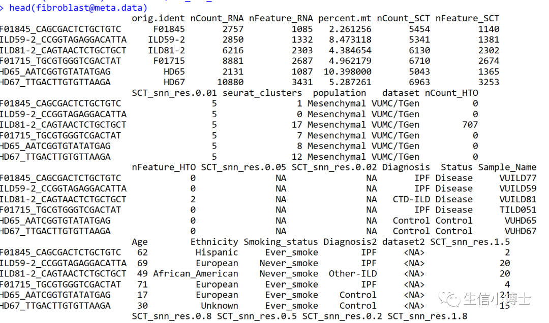
head(subset_rnaslot@meta.data)
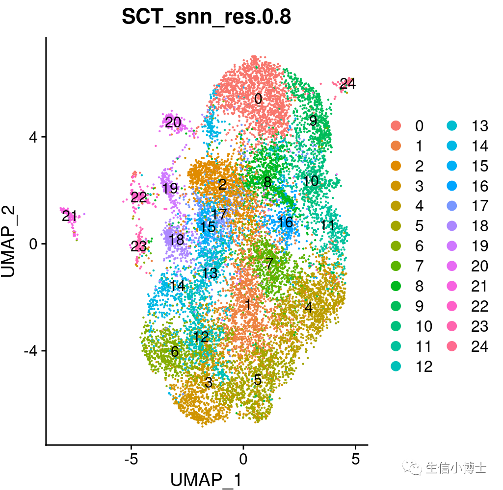
table(subset_rnaslot$SCT_snn_res.0.8)
DimPlot(subset_rnaslot,group.by ="SCT_snn_res.0.8",label = TRUE )
#https://bustools.github.io/BUS_notebooks_R/slingshot.html
library(slingshot)  #https://bioconductor.org/packages/release/bioc/vignettes/slingshot/inst/doc/vignette.html
library(SingleCellExperiment)
library(RColorBrewer)


subset_rnaslot.sce=as.SingleCellExperiment(subset_rnaslot)
head(subset_rnaslot@meta.data)
sds=slingshot(subset_rnaslot.sce,clusterLabels ="cell.type",reducedDim = 'UMAP' ,
              start.clus ="Universal fib")
seu=subset_rnaslot
#sds <- slingshot(Embeddings(seu, "umap"), clusterLabels = seu$seurat_clusters, start.clus = 4, stretch = 0)

sds
summary(sds$slingPseudotime_1)


cell_pal <- function(cell_vars, pal_fun,...) {
  if (is.numeric(cell_vars)) {
    pal <- pal_fun(100, ...)
    return(pal[cut(cell_vars, breaks = 100)])
  } else {
    categories <- sort(unique(cell_vars))
    pal <- setNames(pal_fun(length(categories), ...), categories)
    return(pal[cell_vars])
  }
}
cell_colors <- cell_pal(subset_rnaslot$cell.type, hue_pal())#, brewer_pal("qual", "Set2")
cell_colors_clust <- cell_pal(subset_rnaslot$cell.type, hue_pal())

head(reducedDims(sds)$UMAP)
#head(SlingshotDataSet(sds))
1
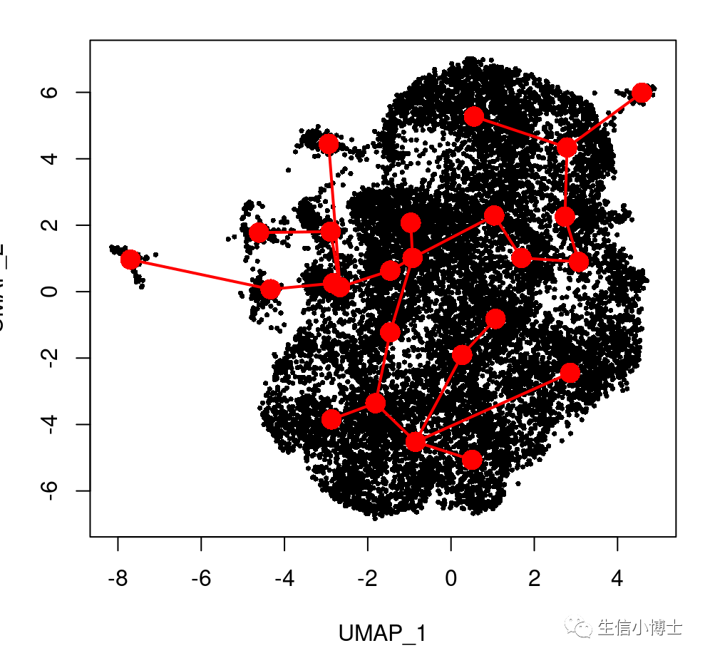
plot(reducedDims(sds)$UMAP, pch = 16, cex = 0.5) #col =brewer.pal("qual", "Set2")[sds$cell_type] ,
lines(SlingshotDataSet(sds), lwd = 2, type = 'lineages', col = 'red')
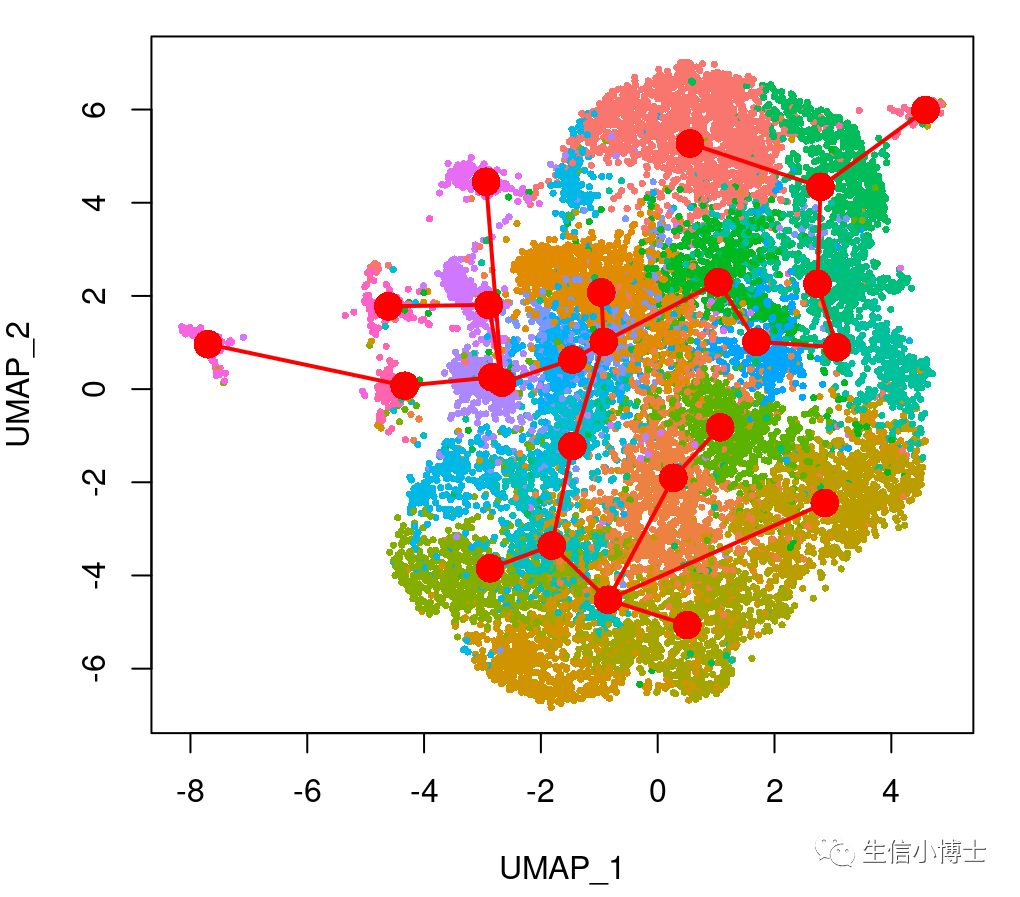
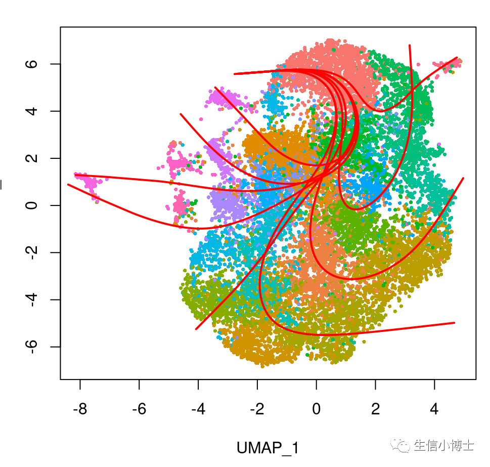
plot(reducedDims(sds)$UMAP,  pch = 16, cex = 0.5, col =cell_colors_clust )
lines(SlingshotDataSet(sds), lwd = 2, type = 'lineages', col = 'red')
得到的拟时序结果
2
plot(reducedDims(sds)$UMAP,pch = 16, cex = 0.5, col =cell_colors_clust )
lines(SlingshotDataSet(sds), lwd = 2, col = 'red')
可以看到细胞的分化轨迹
批量出图
3
pt <- slingPseudotime(sds)
head(pt)
nc <- 3

nms <- colnames(pt)
nr <- ceiling(length(nms)/nc)
nr
pal <- viridis(100, end = 0.95)
c(nr, nc)

par(mfrow = c(nr, nc))

pdf("/home/data/t040413/silicosis/fibroblast_myofibroblast/slingshot/rna/lineages_23.pdf")
for (i in nms) {
  colors <- pal[cut(pt[,i], breaks = 100)]


  plot(reducedDims(sds)$UMAP, col = colors, pch = 16, cex = 0.5, main = i)
  lines(SlingshotDataSet(sds), lwd = 2, col = 'red', type = 'lineages')


}
dev.off()

##########=============或者画一张大图
pdf("/home/data/t040413/silicosis/fibroblast_myofibroblast/slingshot/rna/lineages_2.pdf",width = 20,height = 20)
par(mfrow = c(nr, nc))
for (i in nms) {
  colors <- pal[cut(pt[,i], breaks = 100)]


  plot(reducedDims(sds)$UMAP, col = colors, pch = 16, cex = 0.5, main = i)
  lines(SlingshotDataSet(sds), lwd = 2, col = 'red', type = 'lineages')


}
dev.off()
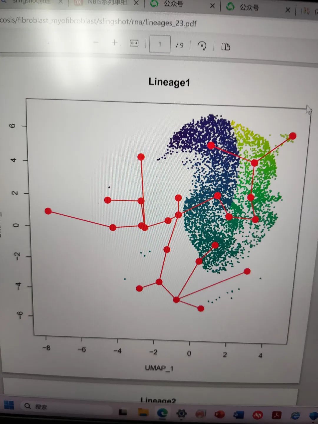
后续是基因的拟时序可视化
4
#差异分析
# Get top highly variable genes
4.1
top_hvg <- HVFInfo(seu) %>%
  mutate(., bc = rownames(.)) %>%
  arrange(desc(residual_variance)) %>%
  top_n(300, residual_variance) %>%
  pull(bc)
head(top_hvg)
# Prepare data for random forest
dat_use <- t(GetAssayData(seu, slot = "data")[top_hvg,])
head(dat_use)[,1:10]
head(slingPseudotime(sds)[,])
dat_use_df <- cbind(slingPseudotime(sds)[,2], dat_use) # Do curve 2, so 2nd columnn
head(dat_use_df)[,1:10]
colnames(dat_use_df)[1] <- "pseudotime"
dat_use_df <- as.data.frame(dat_use_df[!is.na(dat_use_df[,1]),])
head(dat_use_df)[,1:10]

4.2
#The subset of data is randomly split into training and validation; the model fitted on the training set will be evaluated on the validation set.

dat_split <- initial_split(dat_use_df)
dat_split
dat_train <- training(dat_split)
dat_val <- testing(dat_split)
head(dat_val)[,1:10]
dim(dat_train)
dim(dat_val)

4.3
#随机森林模型
#tidymodels is a unified interface to different machine learning models, a “tidier” version of caret. The code chunk below can easily be adjusted to use other random forest packages as the back end, so no need to learn new syntax for those packages.

model <- rand_forest(mtry = 200, trees = 1400, min_n = 15, mode = "regression") %>%
  set_engine("ranger", importance = "impurity", num.threads = 3) %>%
  fit(pseudotime ~ ., data = dat_train)

4.3-1
#模型评价
#The model is evaluated on the validation set with 3 metrics: room mean squared error (RMSE), coefficient of determination using correlation (rsq, between 0 and 1), and mean absolute error (MAE).

val_results <- dat_val %>%
  mutate(estimate = predict(model, .[,-1]) %>% pull()) %>%
  select(truth = pseudotime, estimate)
metrics(data = val_results, truth, estimate)


4.3-2
#RMSE and MAE should have the same unit as the data. As pseudotime values here usually have values much larger than 2, the error isn’t too bad. Correlation (rsq) between slingshot’s pseudotime and random forest’s prediction is very high, also showing good prediction from the top 300 highly variable genes.

summary(dat_use_df$pseudotime)


4.4
#画特定基因
#Now it’s time to plot some genes deemed the most important to predicting pseudotime:
plot(reducedDims(sds)$UMAP, col = colors,
     pch = 16, cex = 0.5, main = top_gene_name[i])
lines(SlingshotDataSet(sds), lwd = 2, col = 'red', type = 'lineages')


var_imp <- sort(model$fit$variable.importance, decreasing = TRUE)
top_genes <- names(var_imp)[1:6]
top_genes
# Convert to gene symbol
top_gene_name <- top_genes#gns$gene_name[match(top_genes, gns$gene)]

par(mfrow = c(3, 2))
for (i in seq_along(top_genes)) {
  colors <- pal[cut(dat_use[,top_genes[i]], breaks = 100)]

  plot(reducedDim(sds), col = colors,
       pch = 16, cex = 0.5, main = top_gene_name[i])
  lines(SlingshotDataSet(sds), lwd = 2, col = 'red', type = 'lineages')
}
dev.off()

pdf("./gene_pseudotime.pdf",width = 12,height = 15)
par(mfrow = c(3, 2))
for (i in seq_along(top_genes)) {
  colors <- pal[cut(dat_use[,top_genes[i]], breaks = 100)]

  plot(reducedDims(sds)$UMAP, col = colors,
       pch = 16, cex = 0.5, main = top_gene_name[i])
  lines(SlingshotDataSet(sds), lwd = 2, col = 'red', type = 'lineages')
}
dev.off()

pdf("./selected_gene_pseudotime.pdf",width = 12,height = 15)
par(mfrow = c(3, 2))
top_gene_name=c("INMT","GPX3","CD34","PI16","SERBP1")
for (i in seq_along(top_genes)) {
  colors <- pal[cut(dat_use[,top_genes[i]], breaks = 100)]

  plot(reducedDims(sds)$UMAP, col = colors,
       pch = 16, cex = 0.5, main = top_gene_name[i])
  lines(SlingshotDataSet(sds), lwd = 2, col = 'red', type = 'lineages')
}
dev.off()

librar

files_tosave= paste(ls(),sep = ",",collapse = ",")
files_tosave
save(files_tosave,file = "/home/data/t040413/silicosis/fibroblast_myofibroblast/slingshot/slingshot.Rdata")
本文参与 腾讯云自媒体同步曝光计划,分享自微信公众号。
原始发表:2023-08-27,如有侵权请联系 cloudcommunity@tencent.com 删除
评论
登录后参与评论
推荐阅读
腾讯云开发者

Copyright © 2013 - 2026 Tencent Cloud. All Rights Reserved. 腾讯云 版权所有
深圳市腾讯计算机系统有限公司 ICP备案/许可证号:粤B2-20090059 ![]() 粤公网安备44030502008569号
粤公网安备44030502008569号
腾讯云计算(北京)有限责任公司 京ICP证150476号 | 京ICP备11018762号