日光性皮炎和银屑病单细胞数据集复现

这周推文更新一篇银屑病相关的单细胞转录组数据的文献复现。使用的SeuratV5版本R包及其常规流程代码。
文章标题:
Single-cell transcriptomics suggest distinct upstream drivers of IL-17A/F in hidradenitis versus psoriasis (J ALLERGY CLIN IMMUNOL)
单细胞转录组学表明,IL-17A/F 在日光性皮炎和银屑病中具有不同的上游驱动力。
文章简介:
背景: 越来越多的证据表明 17T (T17) 细胞和增加的 IL-17 在驱动化脓性汗腺炎 (HS) 病变发展中发挥关键作用。以前在银屑病中使用的生物制剂可阻断 IL-17A 和/或的信号传导 或 IL-17F 同工型已被重新用于治疗 HS。
目的: 研究旨在比较 HS T17 细胞的转录组与银屑病 T17 细胞的转录组,以及它们与邻近免疫细胞亚群的配体-受体相互作用。
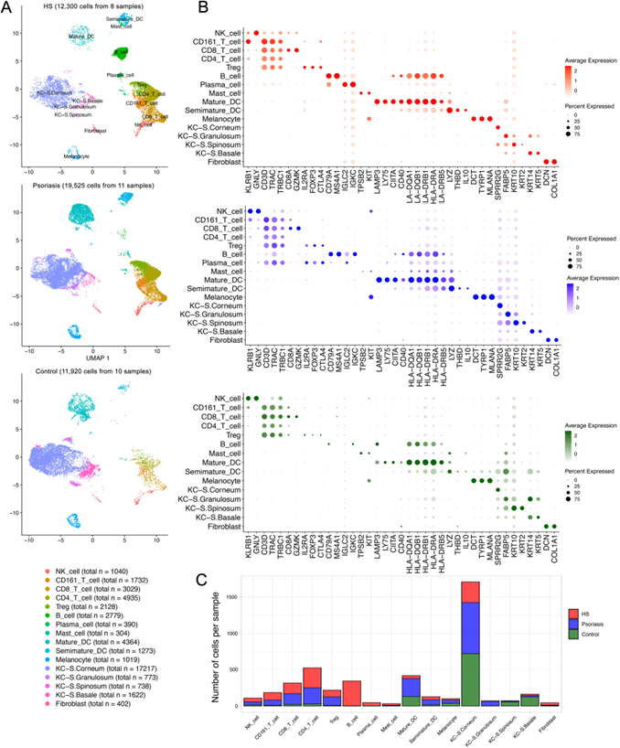
方法: 将来自 8 个去顶手术 HS 皮肤样本(包括真皮隧道)的 12,300 个皮肤免疫细胞的单细胞数据与银屑病皮肤(来自 11 个样本的 19,525 个细胞)和对照皮肤(来自 10 个样本的 11,920 个细胞)的单细胞数据进行比较。
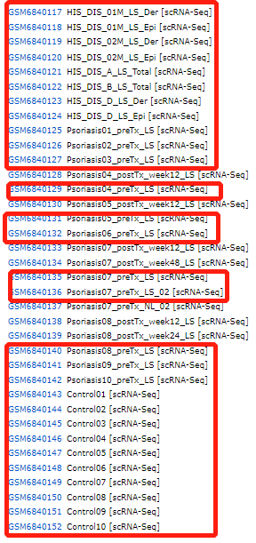
数据集: https://www.ncbi.nlm.nih.gov/geo/query/acc.cgi?acc=GSE220116
所用数据集包括8个HIS,11个Psoriasis,10个control样本。
复现的图:文章主图直接展示的是HS组的亚群细分,但是在做亚群细分之前要先做第一层次的细胞分群,所以这周我先复现第一层次的单细胞转录组数据。
代码
导入数据(10X多样本数据)
rm(list=ls())
options(stringsAsFactors = F)
source('scRNA_scripts/lib.R')
###### step1:导入数据 ######
# https://www.ncbi.nlm.nih.gov/geo/query/acc.cgi?acc=GSE220116
dir='GSE220116/'
fs = list.files('./GSE220116/',pattern = '^GSM')
#执行这一步需要解压tar -xvf
samples=str_split(fs,'_',simplify = T)[,1]
samples
fs
lapply(unique(samples),function(x){
  y=fs[grepl(x,fs)]
  folder=paste0("GSE220116/", str_split(y[1],'_',simplify = T)[,1])
  dir.create(folder,recursive = T)
  #为每个样本创建子文件夹
  file.rename(paste0("GSE220116/",y[1]),file.path(folder,"barcodes.tsv.gz"))
  #重命名文件,并移动到相应的子文件夹里
  file.rename(paste0("GSE220116/",y[2]),file.path(folder,"features.tsv.gz"))
  file.rename(paste0("GSE220116/",y[3]),file.path(folder,"matrix.mtx.gz"))
})
tmp = list.dirs('GSE220116')[-1]
tmp
names(tmp)<-list.dirs("GSE220116",recursive = F)#给orig.ident名字
ct = Read10X(tmp)
ct
sce.all=CreateSeuratObject(counts = ct,
                           min.cells = 5,
                           min.features = 300,)
sce.all
as.data.frame(sce.all@assays$RNA$counts[1:10, 1:2])
head(sce.all@meta.data, 10)
table(sce.all@meta.data$orig.ident)
#HIS1-8;Psoriasis:9-26;Control 27-36
sce.all$group<-ifelse(grepl("GSM6840117|118|119|120|121|122|123|124",sce.all$orig.ident),"HIS",
                  ifelse(grepl("GSM6840143|144|145|146|147|148|149|150|151|152",sce.all$orig.ident),"Control",
                                "Psoriasis"))
table(sce.all$group)
getwd()
1. 质控
###### step2:QC质控 ######
dir.create("./1-QC")
setwd("./1-QC")
# 如果过滤的太狠,就需要去修改这个过滤代码
source('../scRNA_scripts/qc.R')
sce.all.filt = basic_qc(sce.all)
print(dim(sce.all))
print(dim(sce.all.filt))
setwd('../')
table(sce.all.filt$group)
qc.R 代码
basic_qc <- function(input_sce){
  #计算线粒体基因比例
  mito_genes=rownames(input_sce)[grep("^MT-", rownames(input_sce),ignore.case = T)]
  print(mito_genes) #可能是13个线粒体基因
  #input_sce=PercentageFeatureSet(input_sce, "^MT-", col.name = "percent_mito")
  input_sce=PercentageFeatureSet(input_sce, features = mito_genes, col.name = "percent_mito")
  fivenum(input_sce@meta.data$percent_mito)
  #计算核糖体基因比例
  ribo_genes=rownames(input_sce)[grep("^Rp[sl]", rownames(input_sce),ignore.case = T)]
  print(ribo_genes)
  input_sce=PercentageFeatureSet(input_sce,  features = ribo_genes, col.name = "percent_ribo")
  fivenum(input_sce@meta.data$percent_ribo)
  #计算红血细胞基因比例
  Hb_genes=rownames(input_sce)[grep("^Hb[^(p)]", rownames(input_sce),ignore.case = T)]
  print(Hb_genes)
  input_sce=PercentageFeatureSet(input_sce,  features = Hb_genes,col.name = "percent_hb")
  fivenum(input_sce@meta.data$percent_hb)
  #可视化细胞的上述比例情况
  feats <- c("nFeature_RNA", "nCount_RNA", "percent_mito", "percent_ribo", "percent_hb")
  feats <- c("nFeature_RNA", "nCount_RNA")
  p1=VlnPlot(input_sce, group.by = "orig.ident", features = feats, pt.size = 0, ncol = 2) +
    NoLegend()
  p1
  w=length(unique(input_sce$orig.ident))/3+5;w
  ggsave(filename="Vlnplot1.pdf",plot=p1,width = w,height = 5)

  feats <- c("percent_mito", "percent_ribo", "percent_hb")
  p2=VlnPlot(input_sce, group.by = "orig.ident", features = feats, pt.size = 0, ncol = 3, same.y.lims=T) +
    scale_y_continuous(breaks=seq(0, 100, 5)) +
    NoLegend()
  p2
  w=length(unique(input_sce$orig.ident))/2+5;w
  ggsave(filename="Vlnplot2.pdf",plot=p2,width = w,height = 5)

  p3=FeatureScatter(input_sce, "nCount_RNA", "nFeature_RNA", group.by = "orig.ident", pt.size = 0.5)
  ggsave(filename="Scatterplot.pdf",plot=p3)

  #根据上述指标,过滤低质量细胞/基因
  #过滤指标1:最少表达基因数的细胞&最少表达细胞数的基因
  # 一般来说,在CreateSeuratObject的时候已经是进行了这个过滤操作
  # 如果后期看到了自己的单细胞降维聚类分群结果很诡异,就可以回过头来看质量控制环节
  # 先走默认流程即可
  if(F){
    selected_c <- WhichCells(input_sce, expression = nFeature_RNA > 500)
    selected_f <- rownames(input_sce)[Matrix::rowSums(input_sce@assays$RNA$counts > 0 ) > 3]
    input_sce.filt <- subset(input_sce, features = selected_f, cells = selected_c)
    dim(input_sce)
    dim(input_sce.filt)
  }

  input_sce.filt =  input_sce

  # 这里的C 这个矩阵,有一点大,可以考虑随抽样
  C=subset(input_sce.filt,downsample=100)@assays$RNA@layers$counts
  dim(C)
  C=Matrix::t(Matrix::t(C)/Matrix::colSums(C)) * 100

  most_expressed <- order(apply(C, 1, median), decreasing = T)[50:1]

  pdf("TOP50_most_expressed_gene.pdf",width=14)
  boxplot(as.matrix(Matrix::t(C[most_expressed, ])),
          cex = 0.1, las = 1,
          xlab = "% total count per cell",
          col = (scales::hue_pal())(50)[50:1],
          horizontal = TRUE)
  dev.off()
  rm(C)

  #过滤指标2:线粒体/核糖体基因比例(根据上面的violin图)
  selected_mito <- WhichCells(input_sce.filt, expression = percent_mito < 25)
  selected_ribo <- WhichCells(input_sce.filt, expression = percent_ribo > 3)
  selected_hb <- WhichCells(input_sce.filt, expression = percent_hb < 1 )
  length(selected_hb)
  length(selected_ribo)
  length(selected_mito)

  input_sce.filt <- subset(input_sce.filt, cells = selected_mito)
  input_sce.filt <- subset(input_sce.filt, cells = selected_ribo)
  input_sce.filt <- subset(input_sce.filt, cells = selected_hb)
  dim(input_sce.filt)

  table(input_sce.filt$orig.ident)

  #可视化过滤后的情况
  feats <- c("nFeature_RNA", "nCount_RNA")
  p1_filtered=VlnPlot(input_sce.filt, group.by = "orig.ident", features = feats, pt.size = 0, ncol = 2) +
    NoLegend()
  w=length(unique(input_sce.filt$orig.ident))/3+5;w
  ggsave(filename="Vlnplot1_filtered.pdf",plot=p1_filtered,width = w,height = 5)

  feats <- c("percent_mito", "percent_ribo", "percent_hb")
  p2_filtered=VlnPlot(input_sce.filt, group.by = "orig.ident", features = feats, pt.size = 0, ncol = 3) +
    NoLegend()
  w=length(unique(input_sce.filt$orig.ident))/2+5;w
  ggsave(filename="Vlnplot2_filtered.pdf",plot=p2_filtered,width = w,height = 5)
  return(input_sce.filt)

}
2. harmony
#物种是mouse,human要修改sp
sp='human'
# install.packages("Matrix", type = "source")
# install.packages("irlba", type = "source")
###### step3: harmony整合多个单细胞样品 ######
dir.create("2-harmony")
getwd()
setwd("2-harmony")
source('../scRNA_scripts/harmony.R')
# 默认 ScaleData 没有添加"nCount_RNA", "nFeature_RNA"
# 默认的
sce.all.int = run_harmony(sce.all.filt)
setwd('../')
harmony.R的代码
run_harmony <- function(input_sce){

  print(dim(input_sce))
  input_sce <- NormalizeData(input_sce,
                             normalization.method = "LogNormalize",
                             scale.factor = 1e4)
  input_sce <- FindVariableFeatures(input_sce)
  input_sce <- ScaleData(input_sce)
  input_sce <- RunPCA(input_sce, features = VariableFeatures(object = input_sce))
  seuratObj <- RunHarmony(input_sce, "orig.ident")
  names(seuratObj@reductions)
  seuratObj <- RunUMAP(seuratObj,  dims = 1:15,
                       reduction = "harmony")
  input_sce=seuratObj
  input_sce <- FindNeighbors(input_sce, reduction = "harmony",
                             dims = 1:15)
  input_sce.all=input_sce

  #设置不同的分辨率,观察分群效果(选择哪一个?)
  for (res in c(0.01, 0.05, 0.1, 0.2, 0.3, 0.5,0.8,1)) {
    input_sce.all=FindClusters(input_sce.all, #graph.name = "CCA_snn",
                               resolution = res, algorithm = 1)
  }
  colnames(input_sce.all@meta.data)
  apply(input_sce.all@meta.data[,grep("RNA_snn",colnames(input_sce.all@meta.data))],2,table)

  p1_dim=plot_grid(ncol = 3, DimPlot(input_sce.all, reduction = "umap", group.by = "RNA_snn_res.0.01") +
                     ggtitle("louvain_0.01"), DimPlot(input_sce.all, reduction = "umap", group.by = "RNA_snn_res.0.1") +
                     ggtitle("louvain_0.1"), DimPlot(input_sce.all, reduction = "umap", group.by = "RNA_snn_res.0.2") +
                     ggtitle("louvain_0.2"))
  ggsave(plot=p1_dim, filename="Dimplot_diff_resolution_low.pdf",width = 14)

  p1_dim=plot_grid(ncol = 3, DimPlot(input_sce.all, reduction = "umap", group.by = "RNA_snn_res.0.8") +
                     ggtitle("louvain_0.8"), DimPlot(input_sce.all, reduction = "umap", group.by = "RNA_snn_res.1") +
                     ggtitle("louvain_1"), DimPlot(input_sce.all, reduction = "umap", group.by = "RNA_snn_res.0.3") +
                     ggtitle("louvain_0.3"))
  ggsave(plot=p1_dim, filename="Dimplot_diff_resolution_high.pdf",width = 18)

  p2_tree=clustree(input_sce.all@meta.data, prefix = "RNA_snn_res.")
  ggsave(plot=p2_tree, filename="Tree_diff_resolution.pdf")
  table(input_sce.all@active.ident)
  saveRDS(input_sce.all, "sce.all_int.rds")
  return(input_sce.all)
}
3. 降维分群
###### step4: 降维聚类分群和看标记基因库 ######
# 原则上分辨率是需要自己肉眼判断,取决于个人经验
# 为了省力,我们直接看  0.1和0.8即可
table(Idents(sce.all.int))
table(sce.all.int$seurat_clusters)
table(sce.all.int$RNA_snn_res.0.1)
table(sce.all.int$RNA_snn_res.0.8)

p_umap=DimPlot(sce.all.int, reduction = "umap", group.by = "group",label = T,label.box = T);p_umap
getwd()
dir.create('check-by-0.8')
setwd('check-by-0.8')
sel.clust = "RNA_snn_res.0.8"
sce.all.int <- SetIdent(sce.all.int, value = sel.clust)
table(sce.all.int@active.ident)
source('../scRNA_scripts/check-all-markers.R')
setwd('../')
getwd()
所用marker gene
GSE220116gene<-c("KLRB1,GNLY,CD3D,TRAC,TRBC1,CD8A,GZMK,IL2RA,FOXP3,CTLA4,CD79A,MS4A1,IGLC2,IGKC,TPSB2,KIT,LAMP3,LY75,CIITA,CD40,LA-DQA1,LA-DQB1,LA-DRB1,HLA-DRA,LA-DRB5,LYZ,THBD,IL10,DCT,TYRP1,MLANA,SPRR2G,FABP5,KRT10,KRT2,KRT14,KRT5,DCN,COL1A1")
GSE220116gene2<-str_split(GSE220116gene,",")
GSE220116gene3<-unlist(GSE220116gene2)
GSE220116gene3

last_markers = c('PTPRC', 'CD3D', 'CD3E', 'CD4','CD8A',
                   'CD19', 'CD79A', 'MS4A1' ,
                   'IGHG1', 'MZB1', 'SDC1',
                   'CD68', 'CD163', 'CD14',
                   'TPSAB1' , 'TPSB2',  # mast cells,
                   'RCVRN','FPR1' , 'ITGAM' ,
                   'C1QA',  'C1QB',  # mac
                   'S100A9', 'S100A8', 'MMP19',# monocyte
                   'FCGR3A',
                   'LAMP3', 'IDO1','IDO2',## DC3
                   'CD1E','CD1C', # DC2
                   'KLRB1','NCR1', # NK
                   'FGF7','MME', 'ACTA2', ## human  fibo
                 'GJB2', 'RGS5',
                   'DCN', 'LUM',  'GSN' , ## mouse PDAC fibo
                   'MKI67' , 'TOP2A',
                   'PECAM1', 'VWF',  ## endo
                 "PLVAP",'PROX1','ACKR1','CA4','HEY1',
                   'EPCAM' , 'KRT19','KRT7', # epi
                   'FYXD2', 'TM4SF4', 'ANXA4',# cholangiocytes
                   'APOC3', 'FABP1',  'APOA1',  # hepatocytes
                   'Serpina1c',
                   'PROM1', 'ALDH1A1' )

markers = c("GSE220116gene3",
            'last_markers' )

p_umap=DimPlot(sce.all.int, reduction = "umap",label = T,repel = T)
p_umap

if(sp=='human'){
   lapply(markers, function(x){
     #x=markers[1]
     genes_to_check=str_to_upper(get(x))
     DotPlot(sce.all.int , features = genes_to_check )  +
       coord_flip() +
       theme(axis.text.x=element_text(angle=45,hjust = 1))

     h=length( genes_to_check )/6+3;h
     ggsave(paste('check_for_',x,'.pdf'),height = h)
   })

  last_markers_to_check <- str_to_upper(last_markers )

 }else if(sp=='mouse'){
   lapply(markers, function(x){
     #x=markers[1]
     genes_to_check=str_to_title(get(x))
     DotPlot(sce.all.int , features = genes_to_check )  +
       coord_flip() +
       theme(axis.text.x=element_text(angle=45,hjust = 1))

     h=length( genes_to_check )/6+3;h
     ggsave(paste('check_for_',x,'.pdf'),height = h)
   })

   last_markers_to_check <- str_to_title(last_markers )
}else {
  print('we only accept human or mouse')
}
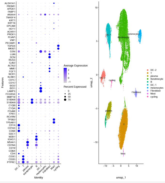
标准亚群命名
sce.all.int
  celltype=data.frame(ClusterID=0:18 ,
                      celltype= 0:18)
  #定义细胞亚群
  celltype[celltype$ClusterID %in% c( 2,4,5,7,8,11,12,15,16 ),2]='Keratinocyte'
  celltype[celltype$ClusterID %in% c( 13 ),2]='Fibroblast'
  celltype[celltype$ClusterID %in% c( 9 ),2]='DC-2'
  celltype[celltype$ClusterID %in% c( 3 ),2]='DC-1'
  celltype[celltype$ClusterID %in% c( 0,1),2]='T'
  celltype[celltype$ClusterID %in% c( 10),2]='melanocytes'
  celltype[celltype$ClusterID %in% c( 17),2]='cycling'
  celltype[celltype$ClusterID %in% c( 14),2]='B'
  celltype[celltype$ClusterID %in% c( 6 ),2]='plasma'
  celltype[celltype$ClusterID %in% c( 18),2]='Mast'
  head(celltype)
  celltype
  table(celltype$celltype)
  sce.all.int@meta.data$celltype = "NA"

  for(i in 1:nrow(celltype)){
    sce.all.int@meta.data[which(sce.all.int@meta.data$RNA_snn_res.0.8 == celltype$ClusterID[i]),'celltype'] <- celltype$celltype[i]}
  Idents(sce.all.int)=sce.all.int$celltype

  table( Idents(sce.all.int))

  sel.clust = "celltype"
  sce.all.int <- SetIdent(sce.all.int, value = sel.clust)
  table(sce.all.int@active.ident)
  p_umap=DimPlot(sce.all.int, reduction = "umap", group.by = "celltype",label = T,label.box = T)
  p_umap

  sp="human"
  dir.create('check-by-celltype')
  setwd('check-by-celltype')
  source('../scRNA_scripts/check-all-markers.R')
  setwd('../')
  getwd()
今天推文代码更新的很完整,大家可以下载数据运行尝试一下。还有一些细节部分没有完全复现,所以下次继续更新这篇文献没有复现的部分。
本文参与 腾讯云自媒体分享计划,分享自微信公众号。
原始发表:2024-04-04,如有侵权请联系 cloudcommunity@tencent.com 删除
评论
登录后参与评论
推荐阅读
目录