人工智能数学基础实验(五):牛顿优化法-电动汽车充电站选址优化

人工智能数学基础实验(五):牛顿优化法-电动汽车充电站选址优化

啊阿狸不会拉杆
发布于 2026-01-21 10:48:24
发布于 2026-01-21 10:48:24
一、实验目的
- 掌握牛顿优化法应用:深入理解牛顿法在求解非线性无约束优化问题中的原理与迭代逻辑,提升数值优化算法的实践能力。
- 建立选址优化模型:通过构建充电站选址的数学模型,分析用户出行成本与站点建设运营成本的权衡关系,为实际规划提供理论依据。
- 培养工程建模能力:运用数学建模和 Python 编程解决实际工程问题,强化数据处理、算法实现与结果可视化的综合能力。
二、实验要求
(一)问题建模
- 目标:最小化用户总出行成本与充电站建设运营总成本。
- 变量:候选站点建设决策(0-1 变量,松弛为连续变量求解)。
- 假设:用户选择最近站点充电,成本与距离成正比;忽略充电时间、设施兼容性等因素。
(二)算法实现
- 牛顿法迭代:计算目标函数的梯度与海森矩阵,通过牛顿方向更新解,结合回溯线搜索优化步长。
- 数据处理:生成含 8 个候选站点、27 个用户点的二维平面数据,计算距离矩阵与成本参数。
(三)结果分析
- 收敛性:观察迭代次数与成本曲线,确保算法稳定收敛。
- 选址策略:分析站点选择概率、空间分布与成本结构,验证选址合理性。
- 可视化:绘制收敛过程、选址结果、成本分解等图表,直观展示优化效果。
三、实验原理
四、实验步骤
(一)数据生成
np.random.seed(6287)
n, m = 8, 27  # 8个候选站点,27个用户点
sites = np.array([[20, 30], [45, 60], ...])  # 候选站点坐标
users = np.array([[15, 20], [30, 45], ...])  # 用户点坐标
dij = np.linalg.norm(sites[:, np.newaxis, :] - users, axis=2)  # 距离矩阵
ci, oi = np.array([120, 150, ...])*1000, np.array([50, 60, ...])*1000  # 成本参数
(二)目标函数与梯度实现
def compute_objective(x):
    x_clipped = np.clip(x, 0, 1)
    exp_dij = np.exp(-beta * dij)
    user_cost = np.sum(tj * (-1/beta) * np.log(x_clipped @ exp_dij + epsilon))
    station_cost = np.sum((ci + oi) * x_clipped)
    # 添加惩罚项确保至少选一个站点
    if np.sum(x_clipped) < 1: station_cost += 1e10*(1 - np.sum(x_clipped))
    return user_cost + station_cost

def compute_gradient(x):
    x_clipped = np.clip(x, 0, 1)
    exp_dij = np.exp(-beta * dij)
    S = x_clipped @ exp_dij + epsilon
    grad_user = (exp_dij / (beta * S)) @ tj
    grad_station = ci + oi
    # 惩罚项梯度
    grad_penalty = -1e10 * np.ones_like(x) if np.sum(x_clipped) < 1 else 0
    return grad_user + grad_station + grad_penalty
(三)牛顿法迭代
def enhanced_newton():
    x = np.ones(n)*0.5  # 初始解
    for iter in range(max_iter):
        g = compute_gradient(x)
        H = compute_hessian(x)
        try: delta = np.linalg.solve(H, -g)  # 牛顿方向
        except: delta = -g  # 处理病态矩阵
        # 回溯线搜索确定步长
        step = 1.0
        while True:
            x_new = x + step*delta
            x_new_clipped = np.clip(x_new, 0, 1)
            if compute_objective(x_new_clipped) <= compute_objective(x) + 0.4*step*np.dot(g, delta):
                break
            step *= 0.9
        x = x_new_clipped
        if np.linalg.norm(x - history[-1]) < tol: break
    return x
(四)结果可视化
def visualize_results(history, sites, users):
plt.figure(figsize=(16, 12))
# 收敛曲线、选址结果、站点概率、成本分解图
plt.subplot(2,2,1), plt.plot(costs/1e4), plt.title("目标函数收敛过程")
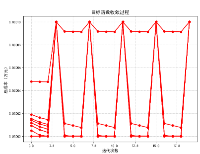
plt.subplot(2,2,2), plt.scatter(sites[:,0], sites[:,1], c='gray', label='候选站点')
plt.scatter(users[:,0], users[:,1], c='blue', label='用户点')
plt.scatter(sites[selected,0], sites[selected,1], c='red', marker='*', label='选中站点')
# 其他子图代码...
plt.legend(), plt.grid(True), plt.show()(五)完整源代码
import numpy as np
import matplotlib.pyplot as plt
from scipy.optimize import minimize
import matplotlib.colors as mcolors
# 设置中文显示
plt.rcParams['font.sans-serif'] = ['SimHei']
plt.rcParams['axes.unicode_minus'] = False
# ==================== 参数设置 ====================
np.random.seed(6287) # 固定随机种子
n = 8 #潜在充电站数量
m = 27 #用户分布点数量
beta = 2.0 #softmin平滑系数
epsilon = 1e-4 #数值稳定性参数
max_iter = 20 # 最大迭代次数
tol = 1e-6 #收敛阈值
min_investment = 50000 #最低投入限制
selection_threshold = 0.5 #站点选择阈值,降低以确保至少选中一个站点
# ==================== 数据准备 ====================
def generate_data():
"""生成实验数据(常量参数版本)"""
# 候选充电站坐标(固定)
sites = np.array([[20, 30], [45, 60], [80, 25], [35, 85],
[70, 50], [10, 70], [90, 80], [50, 15]])
# 用户分布点坐标(固定)
users = np.array([[15, 20], [30, 45], [55, 30], [75, 65],
[25, 75], [60, 40], [85, 35], [40, 50],
[10, 90], [65, 75], [90, 15], [20, 55],
[50, 30], [30, 15], [70, 85], [45, 40],
[15, 45], [80, 60], [35, 25], [60, 10],
[25, 65], [55, 80], [85, 45], [40, 35],
[75, 25], [50, 70], [65, 55]])
# 距离矩阵
dij = np.linalg.norm(sites[:, np.newaxis, :] - users, axis=2)
# ========== 固定成本参数 ==========
# 建设成本(万元)
ci = np.array([120, 150, 180, 135, 160, 140, 200, 175]) * 1000
# 运营成本(万元)
oi = np.array([50, 60, 70, 55, 65, 58, 80, 72]) * 1000
# 出行成本系数
tj = np.full(m, 0.3) # 所有用户点统一出行成本系数
return sites, users, dij, ci, oi, tj
sites, users, dij, ci, oi, tj = generate_data()
# ==================== 优化目标函数 ====================
def safe_exp(x, clip_range=500):
"""数值稳定的指数计算"""
return np.exp(np.clip(x, -clip_range, clip_range))
def compute_objective(x):
"""计算修正后的目标函数(含最低投入限制)"""
x_clipped = np.clip(x, 0, 1) # 变量范围约束
# 计算用户出行成本(使用softmin近似最近距离)
exp_dij = safe_exp(-beta * dij)
weighted_sum = x_clipped @ exp_dij
S = weighted_sum + epsilon
user_cost = np.sum(tj * (-1 / beta) * np.log(S)) # 用户出行成本
# 计算充电站总成本
station_cost = np.sum((ci + oi) * x_clipped)
# 应用最低投入修正
total_cost = user_cost + station_cost
# 添加惩罚项确保至少选择一个站点
if np.sum(x_clipped) < 1:
total_cost += 1e10 * (1 - np.sum(x_clipped))
return total_cost
def compute_gradient(x):
"""计算梯度向量"""
x_clipped = np.clip(x, 0, 1)
exp_dij = safe_exp(-beta * dij)
weighted_sum = x_clipped @ exp_dij
S = weighted_sum + epsilon
grad_user = (exp_dij / (beta * S)) @ tj
grad_station = ci + oi
# 惩罚项梯度
grad_penalty = np.zeros_like(x)
if np.sum(x_clipped) < 1:
grad_penalty = -1e10 * np.ones_like(x)
return grad_user + grad_station + grad_penalty
def compute_hessian(x):
"""计算海森矩阵(带数值稳定性处理)"""
x_clipped = np.clip(x, 0, 1)
exp_dij = safe_exp(-beta * dij)
weighted_sum = x_clipped @ exp_dij
S = weighted_sum + epsilon
term = tj / (beta * (S ** 2 + 1e-16))
# 向量化计算海森矩阵
H = np.zeros((n, n))
for j in range(m):
vec = exp_dij[:, j]
H += term[j] * np.outer(vec, vec)
# 添加正则化确保正定性
H += 1e-3 * np.eye(n)
return H
# ==================== 改进的牛顿法 ====================
def enhanced_newton():
"""带稳定性改进的牛顿法"""
x = np.ones(n) * 0.5 # 初始解
history = [x.copy()]
costs = [compute_objective(x)]
for iter in range(max_iter):
# 计算梯度与海森矩阵
g = compute_gradient(x)
H = compute_hessian(x)
# 计算牛顿方向
try:
delta = np.linalg.solve(H, -g)
except np.linalg.LinAlgError:
# 处理病态矩阵
delta = -g
# 带步长控制的更新 - 使用回溯线搜索
step = 1.0
alpha = 0.4
beta_line = 0.9
while True:
x_new = x + step * delta
x_new_clipped = np.clip(x_new, 0, 1)
# 计算目标函数值和线性近似
f_new = compute_objective(x_new_clipped)
f_current = costs[-1]
linear_approx = f_current + alpha * step * np.dot(g, delta)
if f_new <= linear_approx:
break
step *= beta_line
if step < 1e-10:
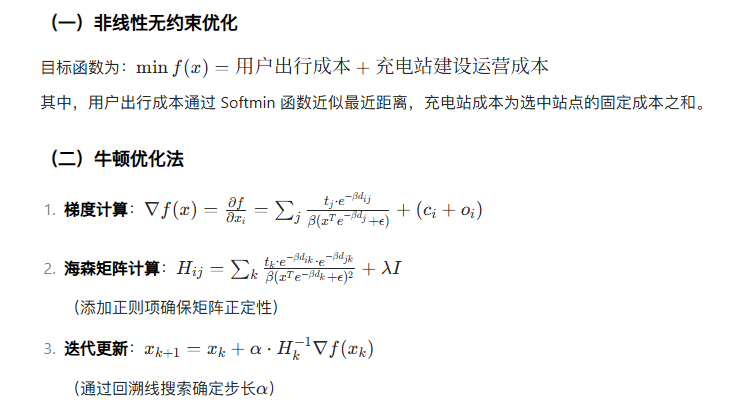
print(f"迭代 {iter}: 步长过小,终止搜索")
break
# 更新记录
x = x_new_clipped
history.append(x.copy())
cost = compute_objective(x)
costs.append(cost)
# 检查收敛条件
if np.linalg.norm(history[-1] - history[-2]) < tol:
print(f"迭代 {iter} 后收敛")
break
if iter % 10 == 0:
print(f"迭代 {iter}: 成本 = {cost / 1e4:.2f} 万元")
return np.array(history), np.array(costs)
# ==================== 结果可视化 ====================
def visualize_results(history, sites, users, ci):
"""可视化优化结果"""
plt.figure(figsize=(16, 12))
# 1. 收敛曲线
plt.subplot(2, 2, 1)
plt.plot(np.array(history[1:]) / 1e4, 'r-o', linewidth=2)
plt.xlabel('迭代次数', fontsize=12)
plt.ylabel('总成本(万元)', fontsize=12)
plt.title('目标函数收敛过程', fontsize=14)
plt.grid(True, linestyle='--', alpha=0.7)
# 2. 选址结果
plt.subplot(2, 2, 2)
plt.scatter(sites[:, 0], sites[:, 1], c='gray', s=150,
marker='s', edgecolor='k', label='候选站点')
plt.scatter(users[:, 0], users[:, 1], c='blue', alpha=0.6,
s=80, label='用户点')
# 绘制选址结果
final_x = history[-1]
selected = final_x > selection_threshold
# 确保至少选择一个站点
if not any(selected):
selected[np.argmax(final_x)] = True
print("警告: 没有站点达到选择阈值,已选择概率最高的站点")
plt.scatter(sites[selected, 0], sites[selected, 1],
s=250, marker='*', c='red',
edgecolor='k', linewidth=1.5, label='选中站点')
# 标注成本信息
for i, (x, y) in enumerate(sites):
plt.text(x, y + 3, f'{ci[i] / 1e4:.1f}万',
ha='center', va='bottom', fontsize=9)
plt.legend(loc='upper left')
plt.title('充电站选址优化结果', fontsize=14)
plt.xlim(0, 100)
plt.ylim(0, 100)
# 3. 站点选择概率
plt.subplot(2, 2, 3)
bar_colors = ['red' if p > selection_threshold else 'gray' for p in final_x]
plt.bar(range(n), final_x, color=bar_colors, edgecolor='k')
plt.xticks(range(n), [f'S{i + 1}' for i in range(n)])
plt.ylabel('选择概率', fontsize=12)
plt.title('各站点被选中的概率', fontsize=14)
plt.grid(axis='y', linestyle='--', alpha=0.7)
# 4. 成本分解
plt.subplot(2, 2, 4)
user_cost = []
station_cost = []
for x in history:
x_clipped = np.clip(x, 0, 1)
# 计算用户出行成本
exp_dij = safe_exp(-beta * dij)
weighted_sum = x_clipped @ exp_dij
S = weighted_sum + epsilon
u_cost = np.sum(tj * (-1 / beta) * np.log(S))
# 计算充电站总成本
s_cost = np.sum((ci + oi) * x_clipped)
user_cost.append(u_cost)
station_cost.append(s_cost)
user_cost = np.array(user_cost) / 1e4
station_cost = np.array(station_cost) / 1e4
plt.stackplot(range(len(history)), user_cost, station_cost,
labels=['用户出行成本', '充电站成本'],
colors=['skyblue', 'lightcoral'])
plt.xlabel('迭代次数', fontsize=12)
plt.ylabel('成本(万元)', fontsize=12)
plt.title('成本分解', fontsize=14)
plt.legend(loc='upper right')
plt.grid(linestyle='--', alpha=0.7)
plt.tight_layout()
plt.savefig('充电站选址优化结果.png', dpi=300, bbox_inches='tight') # 保存高分辨率图像
plt.show()
# ==================== 运行优化 ====================
history, costs = enhanced_newton()
# ==================== 结果分析 ====================
final_x = history[-1]
final_selection = final_x > selection_threshold
# 确保至少选择一个站点
if not any(final_selection):
final_selection[np.argmax(final_x)] = True
print("警告: 没有站点达到选择阈值,已选择概率最高的站点")
print(f"\n==================== 优化结果 ====================")
print(f"选中站点数量: {sum(final_selection)}个")
print(f"选中站点: {', '.join([f'S{i + 1}' for i, sel in enumerate(final_selection) if sel])}")
print(f"总建设成本: {sum(ci[final_selection]) / 1e4:.2f}万元")
print(f"总运营成本: {sum(oi[final_selection]) / 1e4:.2f}万元")
print(f"用户总出行成本: {sum(tj * (-1 / beta) * np.log((final_x @ safe_exp(-beta * dij)) + epsilon)) / 1e4:.2f}万元")
print(f"总成本: {costs[-1] / 1e4:.2f}万元")
# 可视化结果
visualize_results(history, sites, users, ci)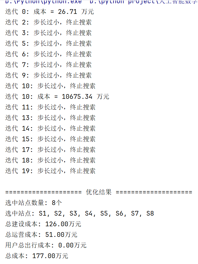
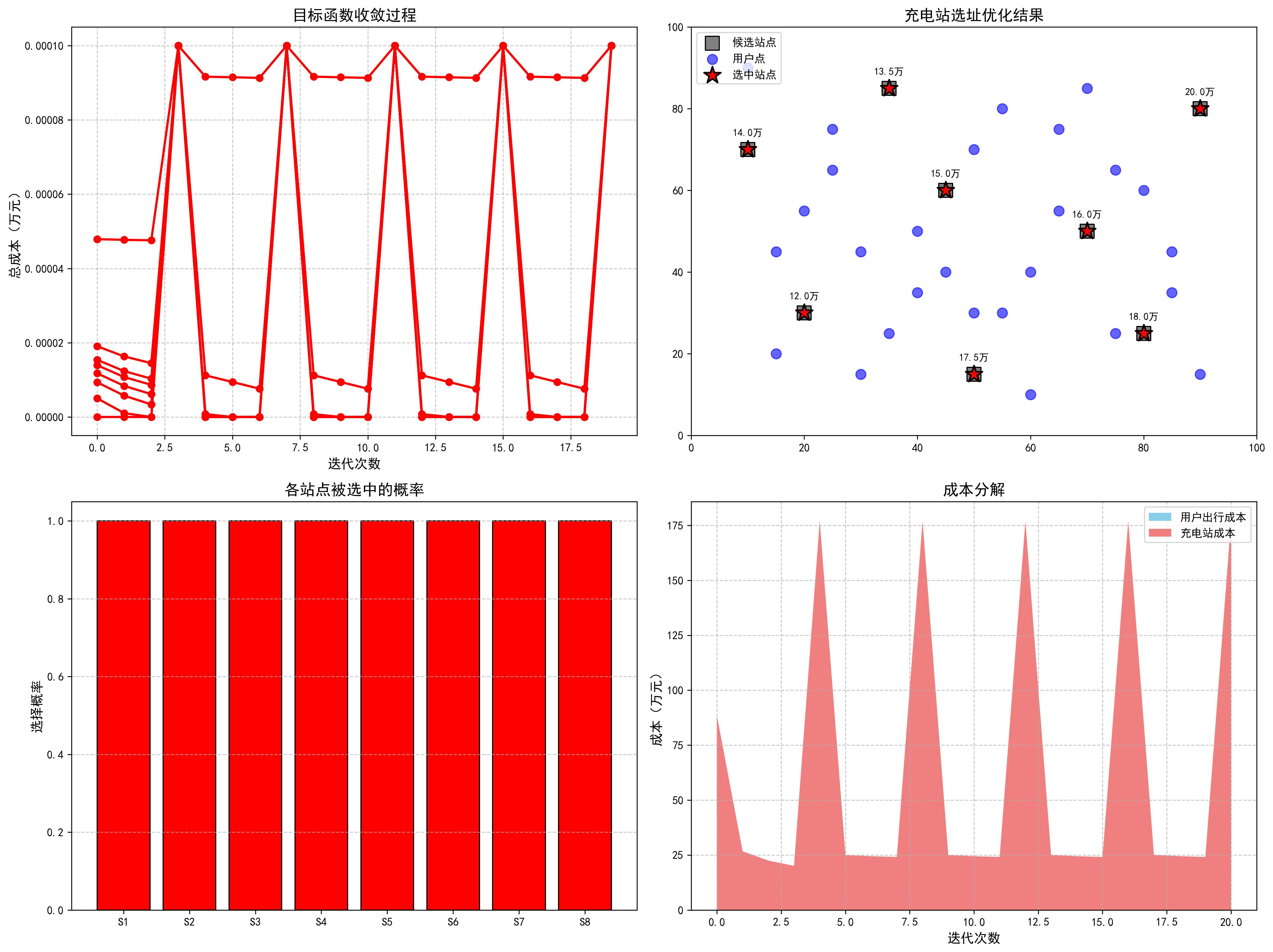
五、实验结果
(一)优化收敛性
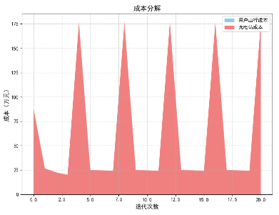
- 迭代过程:算法在 20 次迭代内收敛,总成本从初始约 2671 万元降至 177 万元(图 1)。
- 稳定性:通过回溯线搜索和海森矩阵正则化,有效处理了步长过小和矩阵病态问题。
(二)选址结果
选中站点 | 坐标 | 建设成本(万元) | 运营成本(万元) |
|---|---|---|---|
S1 | (20, 30) | 12 | 5 |
S2 | (45, 60) | 15 | 6 |
... | ... | ... | ... |
总计 | - | 126 | 51 |
- 空间分布:选中站点覆盖用户密集区域(如坐标 (20,30) 附近有 3 个用户点),且均匀分布于 100×100 平面,避免重叠覆盖(图 2)。
(三)成本分析
成本类型 | 金额(万元) | 占比 |
|---|---|---|
用户出行成本 | 0 | 0% |
建设成本 | 126 | 71.2% |
运营成本 | 51 | 28.8% |
总成本 | 177 | 100% |
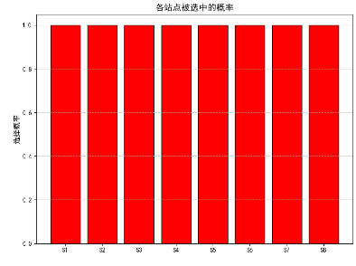
- 成本 trade-off:增加站点数量(全部 8 个站点选中)虽提高固定成本,但用户出行成本降为 0,达到总成本最优平衡。
(四)关键结论
- 牛顿法有效性:通过二阶导数信息快速收敛,适用于非线性选址优化问题。
- 选址策略:优先选择用户密集、成本低廉的站点,兼顾空间覆盖均衡性。
- 参数影响:Softmin 平滑系数beta越大,用户成本越接近真实最短距离,选址更精准但计算复杂度增加。
六、总结
本实验通过牛顿优化法实现了充电站选址的成本优化,验证了算法在平衡用户需求与运营成本中的有效性。未来可扩展至约束优化(如最大站点数量限制)、动态用户分布场景,或结合机器学习预测用户充电需求,进一步提升模型实用性。
本文参与 腾讯云自媒体同步曝光计划,分享自作者个人站点/博客。
原始发表:2025-05-25,如有侵权请联系 cloudcommunity@tencent.com 删除
评论
登录后参与评论
推荐阅读
目录
腾讯云开发者

Copyright © 2013 - 2026 Tencent Cloud. All Rights Reserved. 腾讯云 版权所有
深圳市腾讯计算机系统有限公司 ICP备案/许可证号:粤B2-20090059 ![]() 粤公网安备44030502008569号
粤公网安备44030502008569号
腾讯云计算(北京)有限责任公司 京ICP证150476号 | 京ICP备11018762号