利用单细胞数据对bulk进行反卷积

生信菜鸟团

发布于 2023-10-25 11:33:49

2.8K0

发布于 2023-10-25 11:33:49

文章被收录于专栏：生信菜鸟团生信菜鸟团

intro

buk-RNAseq和sc-RNAseq联合分析在许多文章中已经屡见不鲜了，这周介绍两种利用单细胞数据对bulk进行反卷积方法的基本实现

参考：

这个bulk RNA-seq反卷积工具，你可能还不知道

BayesPrism只有反卷积？那你可能了解的不够多！

单细胞工具-使用BisqueRNA对Bulk RNA-seq数据解卷积

这里沿用BayesPrim的测试数据集，在相同尺度下同时进行BayesPrism和BisqueRNA

两种方法算法原理比较

BayesPrism

BayesPrism方法2022年4月发表在nature cancer(22.7分)

https://www.nature.com/articles/s43018-022-00356-3

https://github.com/Danko-Lab/BayesPrism

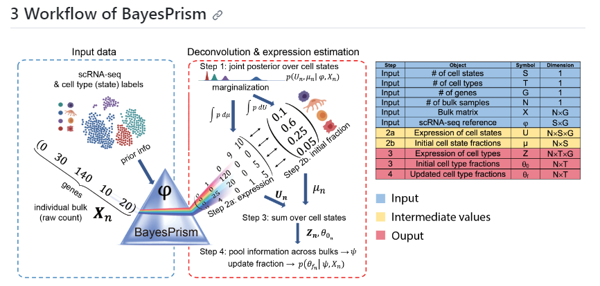
贝叶斯棱镜由Deconvolution modules反卷积模块和Embedding learning module嵌入学习模块组成。反卷积模块对来自scRNA-seq的细胞类型特异性表达谱进行建模，以共同估计肿瘤（或非肿瘤）样品的大量RNA-seq表达的细胞类型组成和细胞类型特异性基因表达的后验分布。嵌入学习模块使用期望最大化（EM）来使用恶性基因程序的线性组合来近似肿瘤表达，同时以反卷积模块估计的非恶性细胞的推断表达和分数为条件。

Deconvolution modules是一种分离混合信号中各个成分的方法。它从单细胞RNA测序(scRNA-seq)中建模先验(cell type-specific expression profiles)的模块。通过对肿瘤(或非肿瘤)样本的批量RNA测序表达进行分析，deconvolution模块可以共同估计细胞类型组成的后验分布和细胞类型特异性基因表达的后验分布。 Embedding learning module则是一个使用期望最大化(Expectation-maximization, EM)算法对肿瘤表达进行建模的模块。它基于先前deconvolution模块推断出的基因表达和非恶性细胞比例的条件下，利用恶性基因程序的线性组合来近似表示肿瘤表达。简单来说，embedding learning module是用来学习肿瘤基因表达的模块，并可以根据先前deconvolution模块的估计结果来进行条件建模。

img

BisqueRNA

BisqueRNA方法2020年发表在NC（16.6分）

https://www.nature.com/articles/s41467-020-15816-6

https://github.com/cozygene/bisque

Bisque 提供两种操作模式：基于参考（单细胞数据集，假设和bulk来自同一样本组织）和基于标记（细胞类型及其marker，属于半监督模型，效果没有参考的好）的分解

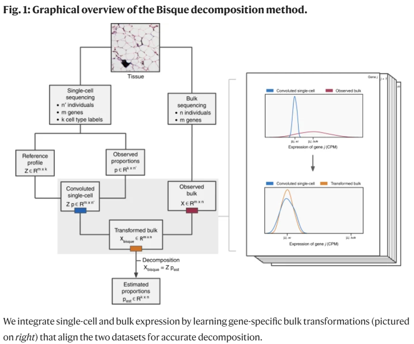
涉及以下步骤：

构建参考图谱：首先，需要构建一个参考图谱，其中包含每种细胞类型的基因表达模式。参考图谱可以从已知的单细胞RNA-seq数据中获取，其中每个细胞单元都被分配给特定的细胞类型。
根据参考图谱反卷积：接下来，将批量RNA-seq数据与参考图谱进行比较，并使用数学算法进行计算，以确定批量数据中每种细胞类型的贡献比例。这个过程可以类比为一个反卷积问题，其中批量数据被视为观测到的总体数据，参考图谱被视为已知的组成部分。
非负最小二乘回归：在BisqueRNA中，使用非负最小二乘回归方法来进行反卷积。这意味着在估计细胞类型比例时，结果必须保持非负且最小误差。非负最小二乘回归是一种优化算法，通过最小化实际数据与估计结果之间的误差来实现这一点。
约束比例总和为一：为了确保估计的细胞类型比例总和为一，还会添加一个约束条件。这样可以保证细胞类型比例之和等于100%，表示完整的细胞组成。

通过这样的反卷积过程，BisqueRNA能够基于批量RNA-seq数据估计出细胞类型的比例，从而提供了对样本中细胞异质性的洞察。这种方法在细胞组成分析中具有广泛的应用，并为我们理解组织和疾病发展提供了重要的信息。

总的来说这类bulk反卷积方法往往需要一个定义好细胞亚型类型的单细胞基因表达谱数据或者定义好细胞亚型的markers列表，就可以对bulk-RNAseq表达谱数据进步性反卷积，得到每个bulk样本中的细胞组成比例估计

其它bulk反卷积方法可参考：

Benchmarking of cell type deconvolution pipelines for transcriptomics data [https://www.nature.com/articles/s41467-020-19015-1]

Benchmarking and new generative methods for single-cell transcriptome data in bulk RNA sequence deconvolution [https://www.researchsquare.com/article/rs-3338396/v1]

BayesPrim

加载数据集

library("devtools")
# install_github("Danko-Lab/BayesPrism/BayesPrism")
# install.packages("BayesPrism/BayesPrism/",repos = NULL, type = "source")
suppressWarnings(library(BayesPrism))

###### 加载数据集 ########
load("./tutorial.gbm.rdata")
ls()
# [1] "bk.dat"            "cell.state.labels" "cell.type.labels"  "sc.dat"

bk.dat[1:4,1:4]
# ENSG00000000003.13 ENSG00000000005.5 ENSG00000000419.11 ENSG00000000457.12
# TCGA-06-2563-01A-01R-1849-01               5033                12               1536                646
# TCGA-06-0749-01A-01R-1849-01               3422                62                934                479
# TCGA-06-5418-01A-01R-1849-01               4976                17               1654                517
# TCGA-06-0211-01B-01R-1849-01               5770                 5               1546                742
# > dim(bk.dat)
# [1]   169 60483
# bulk-RNAseq 基因表达矩阵 169个样本

sc.dat[1:4,1:4]
# ENSG00000130876.10 ENSG00000134438.9 ENSG00000269696.1 ENSG00000230393.1
# PJ016.V3                  0                 0                 0                 0
# PJ016.V4                  0                 0                 0                 0
# PJ016.V5                  0                 0                 0                 0
# PJ016.V6                  0                 0                 0                 0
# > dim(sc.dat)
# [1] 23793 60294
# scRNAseq基因表达矩阵 23793个细胞

# bulk和sc都是6w多的基因 所以肯定包括非编码的

table(cell.type.labels)
# cell.type.labels
# endothelial     myeloid       oligo    pericyte       tcell       tumor 
# 492        2505         160         489          67       20080 
# 已经分好的细胞类型
# > length(cell.type.labels)
# [1] 23793
# 和sc.dat中23793个细胞对应

table(cell.state.labels)
# cell.state.labels
# endothelial     myeloid_0     myeloid_1     myeloid_2     myeloid_3     myeloid_4     myeloid_5     myeloid_6     myeloid_7     myeloid_8 
# 492           550           526           386           382           266           141           130            75            49 
# oligo      pericyte PJ016-tumor-0 PJ016-tumor-1 PJ016-tumor-2 PJ016-tumor-3 PJ016-tumor-4 PJ016-tumor-5 PJ016-tumor-6 PJ017-tumor-0 
# 160           489           621           619           481           420           375           308           261           107 
# PJ017-tumor-1 PJ017-tumor-2 PJ017-tumor-3 PJ017-tumor-4 PJ017-tumor-5 PJ017-tumor-6 PJ018-tumor-0 PJ018-tumor-1 PJ018-tumor-2 PJ018-tumor-3 
# 107           101            89            83            64            22           444           429           403           361 
# PJ018-tumor-4 PJ018-tumor-5 PJ025-tumor-0 PJ025-tumor-1 PJ025-tumor-2 PJ025-tumor-3 PJ025-tumor-4 PJ025-tumor-5 PJ025-tumor-6 PJ025-tumor-7 
# 262           113           971           941           630           601           523           421           397           381 
# PJ025-tumor-8 PJ025-tumor-9 PJ030-tumor-0 PJ030-tumor-1 PJ030-tumor-2 PJ030-tumor-3 PJ030-tumor-4 PJ030-tumor-5 PJ032-tumor-0 PJ032-tumor-1 
# 319           236           563           482           425           419           348            73           195           171 
# PJ032-tumor-2 PJ032-tumor-3 PJ032-tumor-4 PJ032-tumor-5 PJ035-tumor-0 PJ035-tumor-1 PJ035-tumor-2 PJ035-tumor-3 PJ035-tumor-4 PJ035-tumor-5 
# 72            62            57            41           512           474           471           435           385           334 
# PJ035-tumor-6 PJ035-tumor-7 PJ035-tumor-8 PJ048-tumor-0 PJ048-tumor-1 PJ048-tumor-2 PJ048-tumor-3 PJ048-tumor-4 PJ048-tumor-5 PJ048-tumor-6 
# 241           150            81           545           463           437           333           303           277           244 
# PJ048-tumor-7 PJ048-tumor-8         tcell 
# 228           169            67
# 貌似在细胞类型上加上细胞状态？进一步分亚型？

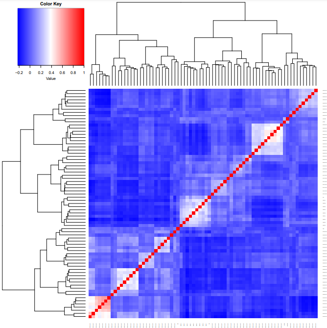
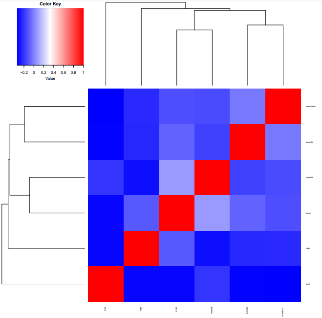
细胞类型和状态标签的 QC

##############细胞类型和状态标签的 QC##############

plot.cor.phi (input=sc.dat,
              input.labels=cell.state.labels,
              title="cell state correlation",
              #specify pdf.prefix if need to output to pdf
              pdf.prefix="gbm.cor.cs",
              cexRow=0.2, cexCol=0.2,
              margins=c(2,2))

plot.cor.phi (input=sc.dat, 
              input.labels=cell.type.labels, 
              title="cell type correlation",
              #specify pdf.prefix if need to output to pdf
              pdf.prefix="gbm.cor.ct",
              cexRow=0.5, cexCol=0.5,
)

# 为进行反卷积cell.type.labels和cell.state.labels要有足够的区分度
# 可以使用使用plot.cor.phi函数查看cell.type.labels和cell.state.labels的特征
# 如果区分度不够或者过了，那么各个群在聚类图中，可能会聚集在一起
# 如果出现大部分cluster 具有明显的相似性，可以考虑merge，或者以更低的resolution进行降维聚类（或者说higher granularity）
# 如果重新聚类或者merge 不合适的话，也可考虑删除

# 可以看到各个标签之间相似度很低

过滤离群基因

#########过滤离群基因############

# 在单细胞测序中，大量的核糖体基因或者线粒体基因不参与指导分析细胞功能，但其可能主导分布并使推断产生偏差。
# 这些基因在区分细胞类型方面通常不能提供信息，并且可能是大的假变异的来源。因此，它们对反卷积是不利的。因此，有必要移除这些基因。

# 查看单细胞数据的离群基因
sc.stat <- plot.scRNA.outlier(
  input=sc.dat, #make sure the colnames are gene symbol or ENSMEBL ID 
  cell.type.labels=cell.type.labels,
  species="hs", #currently only human(hs) and mouse(mm) annotations are supported
  return.raw=TRUE #return the data used for plotting. 
  # pdf.prefix="gbm.sc.stat" # specify pdf.prefix if need to output to pdf
)
head(sc.stat)

# 查看bulk数据的离群基因
bk.stat <- plot.bulk.outlier(
  bulk.input=bk.dat,#make sure the colnames are gene symbol or ENSMEBL ID 
  sc.input=sc.dat, #make sure the colnames are gene symbol or ENSMEBL ID 
  cell.type.labels=cell.type.labels,
  species="hs", #currently only human(hs) and mouse(mm) annotations are supported
  return.raw=TRUE
  #pdf.prefix="gbm.bk.stat" specify pdf.prefix if need to output to pdf
)
head(bk.stat)

# 图中显示每个基因的归一化平均表达(x 轴)和最大特异性(y 轴)的对数，以及每个基因是否属于一个潜在的“异常”
# 可以发现 核糖体蛋白质基因通常表现出高平均表达和低细胞类型特异性得分(局限在右下角)

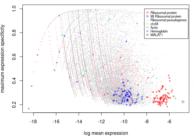
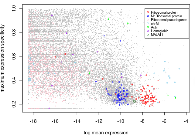
# 查看完之后，将从选定的群体中移除基因。
# 注意，当参考基因和混合基因的性别不同时，建议排除 chrX 和 chrY 基因。
# 也删除低转录基因，因为测量这些基因的转录倾向于噪声。去除这些基因也可以加快计算速度。

sc.dat.filtered <- cleanup.genes (input=sc.dat,
                                  input.type="count.matrix",
                                  species="hs", 
                                  gene.group=c( "Rb","Mrp","other_Rb","chrM","MALAT1","chrX","chrY") ,
                                  exp.cells=5)
# EMSEMBLE IDs detected.
# number of genes filtered in each category: 
#   Rb      Mrp other_Rb     chrM   MALAT1     chrX     chrY 
# 89       78     1011       37        1     2464      594 
# A total of  4214  genes from Rb Mrp other_Rb chrM MALAT1 chrX chrY  have been excluded 
# A total of  24343  gene expressed in fewer than  5  cells have been excluded

dim(sc.dat.filtered)
# [1] 23793 31737
# 只剩下3w多基因了，其实这个过程可以参考我们过去单细胞的过滤，只不过BayesPrism自己也有对应的函数

########检查bulk和sc不同类型基因表达的一致性########

plot.bulk.vs.sc (sc.input = sc.dat.filtered,
                 bulk.input = bk.dat
                 #pdf.prefix="gbm.bk.vs.sc" specify pdf.prefix if need to output to pdf
)

# 这个包有些函数还挺方便的，比如以后检查同一问题不同研究的表达矩阵就可以直接用这个

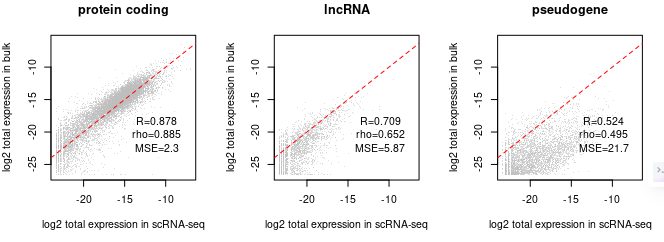
确定bulk RNAseq反卷积的子集

# 从前面的相关性图可以看出来，蛋白质编码基因是两个测定之间最一致的组，那么直接拿蛋白质编码基因子集反卷积是没问题的

sc.dat.filtered.pc <-  select.gene.type (sc.dat.filtered,
                                         gene.type = "protein_coding")
# EMSEMBLE IDs detected.
# number of genes retained in each category: 
#   
#   protein_coding 
# 16148 

# 当观察到严重的批次效应或者在第二步QC时发现一些细胞类型存在非常相似的表达特征时
# 可以考虑使用signature gene
# 特征基因的选择可以丰富用于反卷积的基因信息，同时减少技术批量效应造成的噪声影响

# # Select marker genes (Optional)
# # performing pair-wise t test for cell states from different cell types
# diff.exp.stat <- get.exp.stat(sc.dat=sc.dat[,colSums(sc.dat>0)>3],# filter genes to reduce memory use
#                               cell.type.labels=cell.type.labels,
#                               cell.state.labels=cell.state.labels,
#                               pseudo.count = 0.1, #a numeric value used for log2 transformation. =0.1 for 10x data, =10 for smart-seq. Default=0.1.
#                               cell.count.cutoff=50, # a numeric value to exclude cell state with number of cells fewer than this value for t test. Default=50.
#                               n.cores=1 #number of threads
# )
# # cell.count.cutoff=50
# # 理想情况下，每种细胞类型最好选择足够数量的基因，否则会降低截止值
# # 根据signature gene提取Count matrix subset：
# sc.dat.filtered.pc.sig <- select.marker (sc.dat=sc.dat.filtered.pc,
#                                          stat=diff.exp.stat,
#                                          pval.max=0.01,
#                                          lfc.min=0.1)

构建Prism 对象

# Prism对象包含运行 BayesPrism 所需的所有数据，即 scRNA-seq reference 矩阵、每行参考的 cell type and cell state labels 以及mixture（Bulk RNA-seq）

myPrism <- new.prism(
  reference=sc.dat.filtered.pc, 
  mixture=bk.dat,
  input.type="count.matrix", # 当使用 scRNA-seq  Count 矩阵作为input (推荐)时，用户需要指定 input.type = “ count. Matrix”。Type 的另一个选项是“ GEP”(gene expression profile) ，它是基因矩阵的细胞状态。当使用Bulk RNAseq的数据作为reference 时， 应设置input.type ='GEP'
  cell.type.labels = cell.type.labels, 
  cell.state.labels = cell.state.labels,
  key="tumor",# 参数key是 cell.type.label 中对应于恶性细胞类型的字符向量。如无恶性细胞，即设置为 NULL，此时，所有类型的细胞将被 treated equally
  outlier.cut=0.01,
  outlier.fraction=0.1,
)

运行 BayesPrism

bp.res <- run.prism(prism = myPrism, n.cores=24)  # 24核并行
# Run Gibbs sampling... 
# Current time:  2023-10-16 14:02:06 
# Estimated time to complete:  1hrs 17mins 
# Estimated finishing time:  2023-10-16 15:18:15 
# Start run... 
# R Version:  R version 4.2.2 (2022-10-31) 
# 
# snowfall 1.84-6.2 initialized (using snow 0.4-4): parallel execution on 24 CPUs.
# 
# Stopping cluster
# 
# Update the reference matrix ... 
# snowfall 1.84-6.2 initialized (using snow 0.4-4): parallel execution on 24 CPUs.
# 
# Stopping cluster
# 
# Run Gibbs sampling using updated reference ... 
# Current time:  2023-10-16 14:40:44 
# Estimated time to complete:  38mins 
# Estimated finishing time:  2023-10-16 15:18:17 
# Start run... 
# snowfall 1.84-6.2 initialized (using snow 0.4-4): parallel execution on 24 CPUs.
# 
# Stopping cluster

bp.res
# > slotNames(bp.res)
# [1] "prism"                       "posterior.initial.cellState" "posterior.initial.cellType"  "reference.update"            "posterior.theta_f"  
# [6] "control_param" 

# extract posterior mean of cell type fraction theta
theta <- get.fraction (bp=bp.res,
                       which.theta="final",
                       state.or.type="type")
# > head(theta)
# tumor    myeloid     pericyte endothelial        tcell        oligo
# TCGA-06-2563-01A-01R-1849-01 0.8392297 0.04329259 2.999022e-02  0.07528272 6.474488e-04 0.0115573149
# TCGA-06-0749-01A-01R-1849-01 0.7090654 0.17001073 8.995526e-07  0.01275526 1.179331e-06 0.1081665709
# TCGA-06-5418-01A-01R-1849-01 0.8625322 0.09839143 9.729268e-03  0.02416954 7.039913e-07 0.0051768589
# TCGA-06-0211-01B-01R-1849-01 0.8893449 0.04482991 1.131622e-02  0.05435490 2.508238e-06 0.0001515524
# TCGA-19-2625-01A-01R-1850-01 0.9406438 0.03546026 1.932740e-03  0.01309753 4.535897e-06 0.0088610997
# TCGA-19-4065-02A-11R-2005-01 0.6763166 0.08374439 1.849921e-01  0.01918132 3.541126e-04 0.0354114398
# > dim(theta)
# [1] 169   6

在BayesPrim基础上我们使用相同的蛋白质编码基因子集通过BisqueRNA进行反卷积

BisqueRNA

准备数据

# install.packages("BisqueRNA")
library(Biobase)
library(BisqueRNA)

# bulk
bk.dat[1:4,1:4]
bulk.matrix <- t(bk.dat)
bulk.eset <- Biobase::ExpressionSet(assayData = bulk.matrix)
bulk.eset@assayData[["exprs"]][1:4,1:4]

# sc
# 统一用蛋白质编码基因
sc.dat.filtered.pc[1:4,1:4]
sc.matrix <- t(sc.dat.filtered.pc)
sc.obj <- Seurat::CreateSeuratObject(counts = sc.matrix)
# sc.dat.filtered.pc对象前面已经过滤了，这里就不根据min.cell min.features等参数过滤、
sc.obj@assays$RNA@counts[1:4,1:4]
# 如果单细胞数据（来自 10x 平台）在seurat中，且包含细胞类型信息，Bisque 包含一个函数，该函数会自动将此对象转换为表达式集
sc.eset <- BisqueRNA::SeuratToExpressionSet(sc.obj, delimiter="\\.", position=1, version="v3")  # delimiter分割，postion指定样本id
# Split sample names by "\." and checked position 1. Found 8 individuals.
# Example: "PJ016.V3" corresponds to individual "PJ016".
table(sc.eset$SubjectName)
# PJ016 PJ017 PJ018 PJ025 PJ030 PJ032 PJ035 PJ048 
# 3085  1261  2197  5924  3097  1377  3768  3084 
# 包含8个独立样本

# 加入细胞类型
table(cell.type.labels)
sc.eset$cellType <- cell.type.labels
table(sc.eset$cellType)
# endothelial     myeloid       oligo    pericyte       tcell       tumor 
# 492        2505         160         489          67       20080

基于参考数据集的分解

# 因为我们拿到BisqueRNA里来的矩阵就已经是蛋白质编码的了
# 所以这里其实就是进行类似BayesPrism里的蛋白质子集的反卷积
res <- BisqueRNA::ReferenceBasedDecomposition(bulk.eset, sc.eset, markers=NULL, use.overlap=FALSE)

# 如果bulk和单细胞数据是同一个样本测得，可以设置use.overlap=TRUE，可能有更好的表现
# 但如果不同数据集样本强行use.overlap=TRUE：
# Decomposing into 6 cell types.
# Error in GetOverlappingSamples(sc.eset, bulk.eset, subject.names, verbose) : 
#   No overlapping samples in bulk and single-cell expression.

ref.based.estimates <- t(res$bulk.props)
head(ref.based.estimates)
library(tidyverse)
# 根据BayesPrim结果顺序排序
estimates <- as.data.frame(ref.based.estimates) %>% select(tumor,myeloid,pericyte,endothelial,tcell,oligo) %>% as.matrix()
head(estimates)

head(theta)

dim(estimates);dim(theta)
# [1] 169   6
# [1] 169   6

此外，当没有参考单细胞数据集时，BisqueRNA可以仅使用已知的标记基因提供相对细胞类型丰度的估计值

这其实是一个比较灵活的接口了，如果我们想使用像在前面BayesPrism提到的signature gene进行反卷积，也可以通过这个接口进行调整

详情参考原介绍BisqueRNA的推文

简单比较BayesPrism和BisqueRNA的结果

# 同一细胞类型样本间比较
tmp <- c()
for (i in seq(1,6)){
  tmp <- c(tmp, cor(estimates[,i],theta[,i]))
}
tmp
# tumor,myeloid,pericyte,endothelial,tcell,oligo
# [1] 0.8388819 0.9704178 0.3984573 0.2961502 0.1585450 0.2849336

# 同一样本细胞类型占比比较
tmp <- c()
for (i in seq(1,169)){
  tmp <- c(tmp, cor(estimates[i,],theta[i,]))
}
tmp
range(tmp)
# [1] 0.7806862 0.9998643

以上就是本周转录组周更的全部内容

本文参与腾讯云自媒体同步曝光计划，分享自微信公众号。

原始发表：2023-10-24，如有侵权请联系 cloudcommunity@tencent.com 删除

cell