BD单细胞测序数据分析流程（全）

生信菜鸟团

发布于 2024-04-11 15:04:29

1590

发布于 2024-04-11 15:04:29

文章被收录于专栏：生信菜鸟团生信菜鸟团

前言

BD和10x是两种常见的单细胞测序技术平台。我们已经分享了很多的10x 测序的教程。

但是目前中文平台中关于BD公司的单细胞测序介绍较少，暂无完整的中文分析教程，今天我们来分享全流程的BD单细胞测序数据分析。

BD：BD公司的单细胞测序技术采用了特殊的芯片和试剂盒，测序数据通常需要通过BD公司提供的分析软件进行预处理，包括数据质控、细胞识别和基因表达估计等步骤。
10x：10x Genomics提供的单细胞测序技术通常使用其独特的微流控芯片和试剂盒，测序数据可以使用10x Genomics提供的Cell Ranger等分析软件进行预处理。与BD相比，10x的数据预处理流程有所不同。

但是这些预处理步骤，我们可以不去过多的关心，因为预处理的数据通常都是下机之后，公司会交给我们的，我们只用继续下游的分析即可。

如果你对BD的预处理比较感兴趣，可以参考：BD单细胞测序手册

本篇推文的上一集内容：BD单细胞转录组分析怕不是一个笑话吧

GSE201088

下载数据

首先我们下载数据

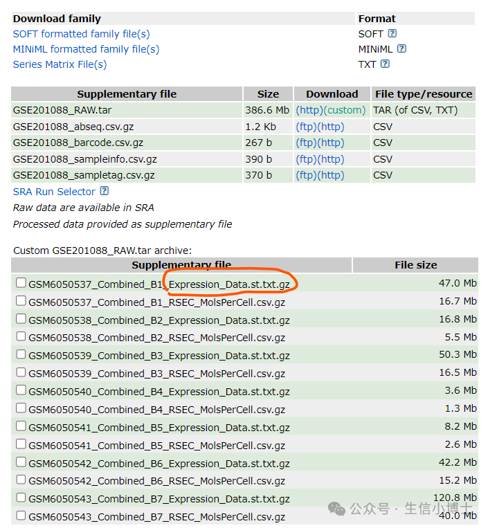
1 geo里面数据存放如下

2 如果，你也想高速下载geo其他的数据，使用下面的代码百试不爽

cd 20240405_gse201088_pbmc_covid/
nohup wget -c -nd --cut-dirs=4 ftp://ftp.ncbi.nlm.nih.gov/geo/series/GSE201nnn/GSE201088/suppl/*  &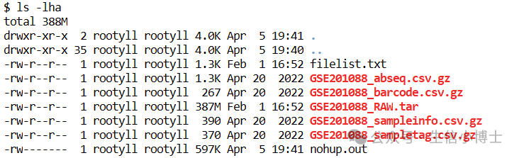

3 然后解压

tar -xvf  GSE201088_RAW.tar 
ls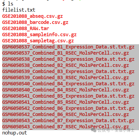

读取BD单个样本

1 在r中读取并理解数据

# 导入必要的包
library(data.table)
dir.create("~/gzh/20240405_gse201088_pbmc_covid/")
setwd('~/gzh/20240405_gse201088_pbmc_covid/')


# 读取.gz文件
file_path <- "GSM6050537_Combined_B1_Expression_Data.st.txt.gz"
data <- data <- fread(file_path)
table(data$Cell_Index)


barcodes=fread("GSE201088_barcode.csv.gz")
abseq=fread('GSE201088_abseq.csv.gz')
mols=fread('GSM6050537_Combined_B1_RSEC_MolsPerCell.csv.gz')

mols[100:108,106:109]
range(mols[,'ABCC9'])

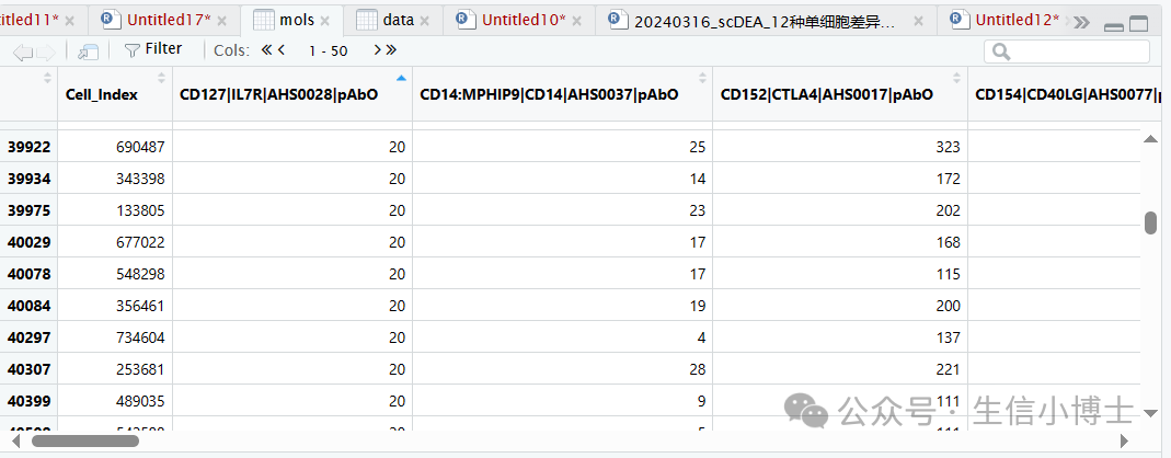
#这个矩阵的前半部分是abseq，后半部分是WAT，所以理论上这两部分可以分别走seurat流程。 #但是abseq只测了40个蛋白，所以感觉更好的办法还是使用reference mapping的方法。 #或者根本就不需要处理abseq，最后把abseq的信息加入WAT对象中即可，这个方法省时省力

具体文件细节可以参考：BD单细胞手册的缩略词部分

2 数据拆分成abseq和WAT

注意矩阵是否需要转置

library(dplyr)

wat= textshape::column_to_rownames(mols,"Cell_Index")    %>% 
                         .[,41:ncol(.)] %>%as.matrix() %>% as(., "dgCMatrix")

library(Seurat)

abseq=textshape::column_to_rownames(mols,"Cell_Index")    %>% 
  .[,1:40]  %>%as.matrix() %>%     as(., "dgCMatrix")

批量读取BD多个样本

1 批量把数据拆分成abseq和WAT，并转为seurat对象

#2 批量把数据拆分成abseq和WAT----

future::plan(future::multisession, workers = 7 ) #有几个任务就设置几个核心

wat_list=list()
abseq_list=list()


# 使用 map 函数处理数据
output_lists <- purrr::map(list.files("./", pattern = "MolsPerCell"),
                                  function(x) {

                                    # 提取样本名
                                    sample_name <- stringr::str_split(string = x, pattern = "_", simplify = TRUE)[, 1]

                                    # 读取数据
                                    mols <- fread(x)

                                    # 处理数据为 wat 和 abseq
                                    wat <- textshape::column_to_rownames(mols, "Cell_Index") %>%
                                      .[, 41:ncol(.)] %>%
                                      as.matrix()      %>%t()     %>%
                                      as(., "dgCMatrix")
                                    abseq <- textshape::column_to_rownames(mols, "Cell_Index") %>%
                                      .[, 1:40] %>%
                                      as.matrix() %>%t()       %>%
                                      as(., "dgCMatrix")

                                    # 创建 Seurat 对象并添加到列表中
                                    wat_list[[sample_name]] <- CreateSeuratObject(counts = wat, project = sample_name, assay = "RNA")
                                    abseq_list[[sample_name]] <- CreateSeuratObject(counts = abseq, project = sample_name, assay = "abseq")

                                    # 返回 wat_list 和 abseq_list
                                    return(list(wat_list = wat_list, abseq_list = abseq_list))
                                  }
)

# 提取 wat_list 和 abseq_list
wat_lists <- purrr::map(output_lists, ~ .x$wat_list)
abseq_lists <- purrr::map(output_lists, ~ .x$abseq_list)

# 合并所有结果
wat_list <- purrr::reduce(wat_lists, c)
abseq_list <- purrr::reduce(abseq_lists, c)

# 保存 wat_list 到文件
saveRDS(wat_list, file = "wat_list.rds")

# 保存 abseq_list 到文件
saveRDS(abseq_list, file = "abseq_list.rds")

2 建立seruat v5对象，并加入样本信息


#建立seurat v5对象,加入样本信息------------
setwd("~/gzh/20240405_gse201088_pbmc_covid/")

wat_list=readRDS("./wat_list.rds")


wat_list

lapply(wat_list,FUN = function(each) {each$orig.ident= Project(each)})



wat= merge(wat_list[[1]],wat_list[-1])
dim(wat)
wat=JoinLayers(wat )
head(wat@meta.data)
wat$sample=wat$orig.ident
wat@assays$RNA@layers$counts[1:9,1:8]
head(rownames(wat))
head(colnames(wat))

sce.all= wat

head(sce.all@meta.data)

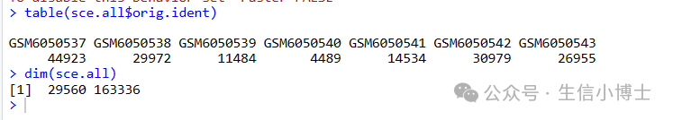
table(sce.all$orig.ident)
dim(sce.all)
head(colnames(sce.all))

harmony单细胞整合流程

1 harmony流程，并检查不同分辨率下的分群情况



###### step2: QC质控 ######
dir.create("./1-QC")
setwd("./1-QC")

# 如果过滤的太狠，就需要去修改这个过滤代码
source('~/OLP_combine/scRNA_scripts/qc.R')
sce.all.filt = basic_qc(sce.all)
print(dim(sce.all))
print(dim(sce.all.filt))
print(getwd())
setwd('../')
sp='human'
getwd()




###### step3: harmony整合多个单细胞样品 ######
#"orig.ident"存储样本信息，按照样本，使用harmony来去除批次效应----
sce.all.filt 
head(sce.all.filt@meta.data)

if(T){
  dir.create("2-harmony")
  getwd()
  setwd("2-harmony")
  source('~/OLP_combine/scRNA_scripts/harmony.R')
  # 默认 ScaleData 没有添加"nCount_RNA", "nFeature_RNA"
  # 默认的
  sce.all.int = run_harmony(sce.all.filt)
  print(getwd())
  setwd('../')

}

###### step4:  看标记基因库 ######
# 原则上分辨率是需要自己肉眼判断，取决于个人经验
# 为了省力，我们直接看  0.1和0.8即可

table(Idents(sce.all.int))
table(sce.all.int$seurat_clusters)
table(sce.all.int$RNA_snn_res.0.1) 
table(sce.all.int$RNA_snn_res.0.8) 

#####整合完成之后，查看0.1分辨率------
getwd()
dir.create('check-by-0.1')
setwd('check-by-0.1')


sce.all.int@meta.data %>%head()
sel.clust = "RNA_snn_res.0.1"

sce.all.int <- SetIdent(sce.all.int, value = sel.clust)
table(sce.all.int@active.ident) 
print(getwd())

source('~/OLP_combine/scRNA_scripts/check-all-markers.R')
setwd('../') 
getwd()


#####整合完成之后，查看0.5分辨率------
dir.create('check-by-0.5')
setwd('check-by-0.5')
sel.clust = "RNA_snn_res.0.5"
sce.all.int <- SetIdent(sce.all.int, value = sel.clust)
table(sce.all.int@active.ident) 
source('~/OLP_combine/scRNA_scripts/check-all-markers.R')
setwd('../') 
getwd()

#####整合完成之后，查看0.8分辨率------
dir.create('check-by-0.8')
setwd('check-by-0.8')
sel.clust = "RNA_snn_res.0.8"
sce.all.int <- SetIdent(sce.all.int, value = sel.clust)
table(sce.all.int@active.ident) 
source('~/OLP_combine/scRNA_scripts/check-all-markers.R')
setwd('../') 
getwd()

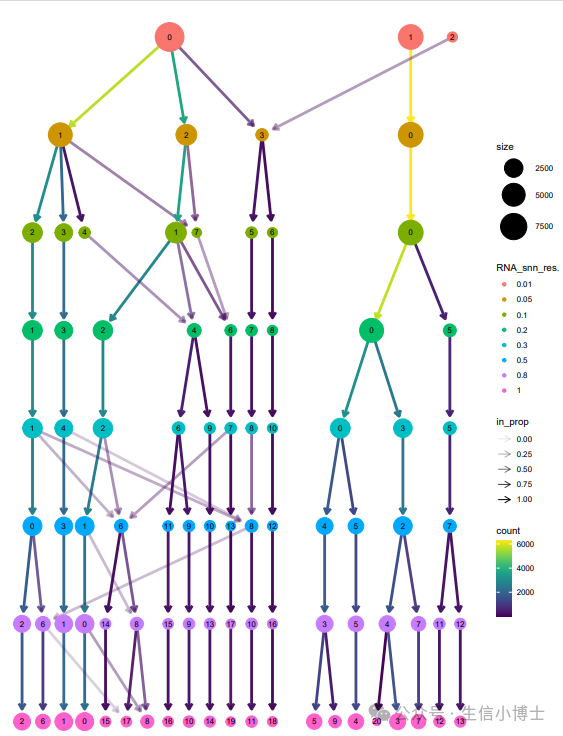
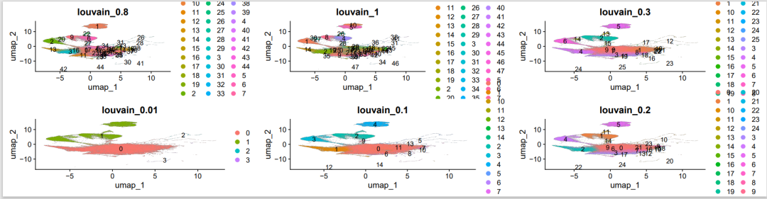
不同分辨率下的分群

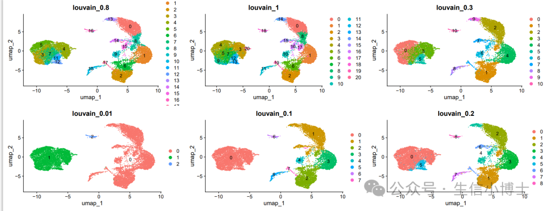
不同分辨率下的ump图展示

我的这个umap图看上去比下面的原图好看多了，不知道啥原因呢？

下面这个为文献里面的原图

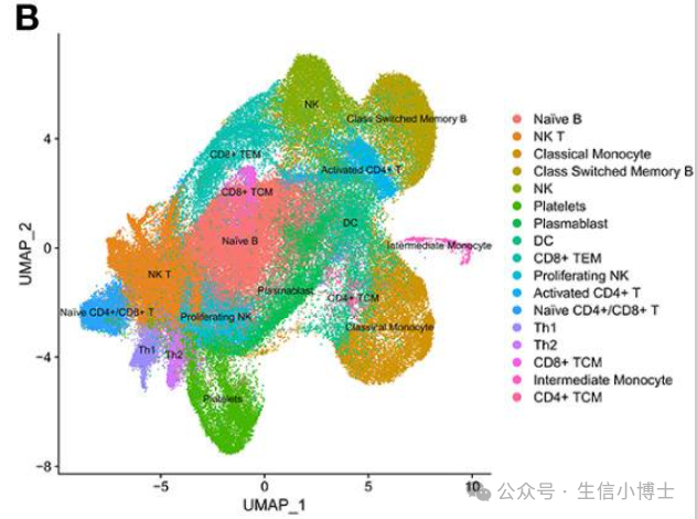
https://www.ncbi.nlm.nih.gov/pmc/articles/PMC9755500/

文献里面用的是SCTransform v2进行批次矫正和标准化。这和我们的方法不同，这可能是umap图变好看的主要原因。（估计作者使用了MNN矫正数据，但是也没看到作者的代码）

原文：post QC of the data quality ( Supplementary File 1 ; Figure S1A ), a total of 124726 cells were retained after removing the low-quality cells. We performed batch effect correction and normalization using Seurat SCTransform v2 (24), followed by dimension reduction and unsupervised clustering using the Louvain algorithm (resolution = 0.4). The cluster specific genes were identified using Seurat FindMarker functions and the clusters were annotated manually using CellMarker, PanglaoDB and Azimuth, as well as using a Support Vector Machine (SVM)-based annotation tool scPred。

单细胞注释

细胞命名

1 0.1分辨率下，共有七个亚群

在这里我们取0.1分辨率时候的分群

# 付费环节 800 元人民币
# 如果是手动给各个单细胞亚群命名----------
if(F){
  sce.all.int
  table(Idents(sce.all.int))
  table(sce.all.int$RNA_snn_res.0.1)
  table(sce.all.int$RNA_snn_res.0.5)


  celltype=data.frame(ClusterID=0:7 ,
                      celltype= 0:7) 
  #定义细胞亚群        
  celltype[ celltype$ClusterID %in% c( 0  ) ,2 ]='Mono' 

  celltype[celltype$ClusterID %in% c( 1 ),2]='B' 
  celltype[celltype$ClusterID %in% c( 2   ),2]= 'T/NK' # 

  celltype[celltype$ClusterID %in% c( 3 ),2]='T'

  celltype[celltype$ClusterID %in% c( 4 ),2]='Mixed'
  celltype[celltype$ClusterID %in% c( 5 ),2]='Prolif'

  celltype[celltype$ClusterID %in% c( 6 ),2]='Plasma'
  celltype[celltype$ClusterID %in% c( 7 ),2]='Megakaryocyte'

  # celltype[celltype$ClusterID %in% c( 9 ),2]='mast' 
  # celltype[celltype$ClusterID %in% c( 8 ),2]='cycle' 
  # celltype[celltype$ClusterID %in% c( 10 ),2]='double'
  # celltype[celltype$ClusterID %in% c( 11 ),2]='Leydig'  #Leydig
  # 
  head(celltype)
  celltype
  table(celltype$celltype)
  sce.all.int@meta.data$celltype = "NA"

  for(i in 1:nrow(celltype)){
    #使用0.1分辨率
    sce.all.int@meta.data[which(sce.all.int@meta.data$RNA_snn_res.0.1 == celltype$ClusterID[i]),'celltype'] <- celltype$celltype[i]}
  table(sce.all.int$celltype)
  Idents(sce.all.int)=sce.all.int$celltype

  }

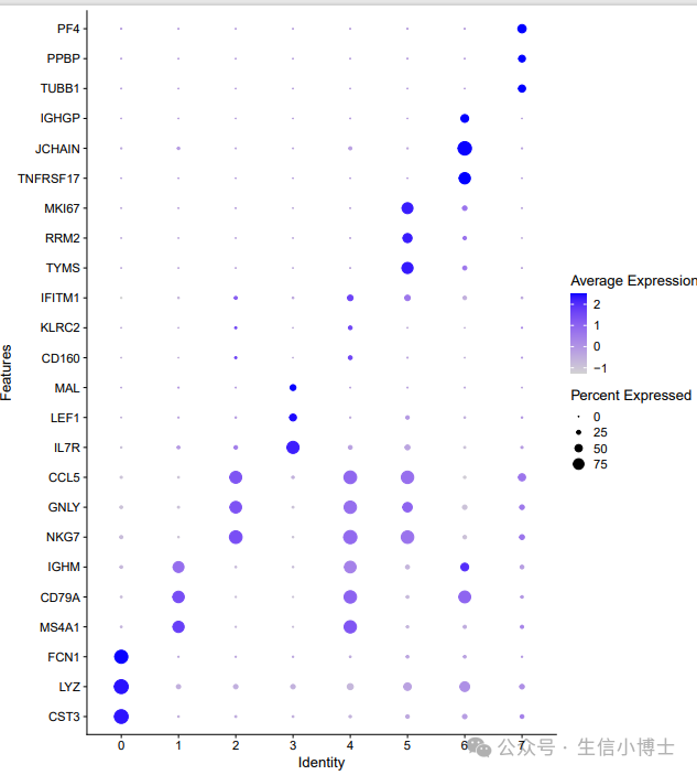
2 命名完之后的dotplot图

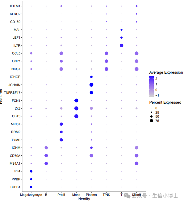
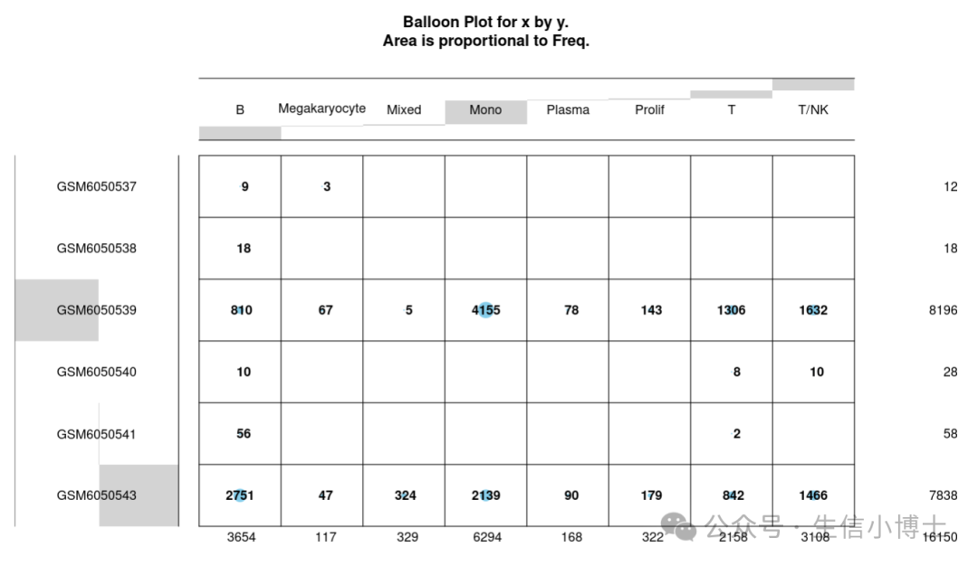
但是这个表格看上去着实有点怪异，所有的细胞基本只在两个GSM里面有测到，这明显不符合常理

原文：PBMCs were isolated from Healthy (n = 4), COVID-19 (n = 16) and recovered (n = 13) individuals, using BD vaccutainers cell prepataion tubes. PBMCs were isolated as per manufacturer's recommendation, and stored for future use. Samples were multiplexed using BD single cell multiplexing kit (Human), followed by tagging with a pool of 40 oligo-attached antibody for surface markers (Ab-Seq). Around 30000 cells were loaded per cartridge, followed by cell lysis, cDNA synthesis and final library preparation using BD WTA amplification kit as per manufacturer's recommendation. A poly-A transcripts library (WTA), Ab-Seq library and library from oligos of Sampe multiplexing kit (SMK) were constructed from each batch, and were sequenced on NovaSeq 6000 platform.

于是我检查一下是不是我的处理有问题

应该是我的质控太严格了，那么我们从质控前的步骤看下seurat对象

input_sce=sce.all

#计算线粒体基因比例
mito_genes=rownames(input_sce)[grep("^MT-", rownames(input_sce),ignore.case = T)] 
print(mito_genes) #可能是13个线粒体基因
#input_sce=PercentageFeatureSet(input_sce, "^MT-", col.name = "percent_mito")
input_sce=PercentageFeatureSet(input_sce, features = mito_genes, col.name = "percent_mito")
fivenum(input_sce@meta.data$percent_mito)

#计算核糖体基因比例
ribo_genes=rownames(input_sce)[grep("^Rp[sl]", rownames(input_sce),ignore.case = T)]
print(ribo_genes)
input_sce=PercentageFeatureSet(input_sce,  features = ribo_genes, col.name = "percent_ribo")
fivenum(input_sce@meta.data$percent_ribo)

#计算红血细胞基因比例
Hb_genes=rownames(input_sce)[grep("^Hb[^(p)]", rownames(input_sce),ignore.case = T)]
print(Hb_genes)
input_sce=PercentageFeatureSet(input_sce,  features = Hb_genes,col.name = "percent_hb")
fivenum(input_sce@meta.data$percent_hb)

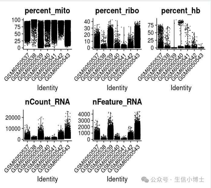
VlnPlot(input_sce,features = c("percent_mito","percent_ribo","percent_hb"),raster=FALSE)

结果发现，下图的线粒体高的吓人，在我第一次质控之后，这些高线粒体表达的细胞都被过滤掉了，所以我只拿到16150个细胞。

我本来还是想继续探索一下这个数据集的，但是看到qc之前的下图这么高的线粒体比例，一下子没了兴趣....

但是既然是全文第一篇全面的bd分析教程，硬着头皮继续走吧

原文中说到a total of 124726 cells were retained after removing the low-quality cells.但是我并没有找到作者的质控标准，所以简单粗暴一点，取线粒体百分比小于90%的细胞，我们就可以得到119360个细胞。代码如下

if (F) {#不进行质控，看最终的umap图--------

  setwd("~/gzh/20240405_gse201088_pbmc_covid/")

  wat_list=readRDS("./wat_list.rds")


  wat_list

  lapply(wat_list,FUN = function(each) {each$orig.ident= Project(each)})



  wat= merge(wat_list[[1]],wat_list[-1])
  dim(wat)
  wat=JoinLayers(wat )
  head(wat@meta.data)
  wat$sample=wat$orig.ident
  wat@assays$RNA@layers$counts[1:9,1:8]
  head(rownames(wat))
  head(colnames(wat))

  sce.all= wat
  input_sce=sce.all
  head(sce.all@meta.data)

  table(sce.all$orig.ident)
  dim(sce.all)
  head(colnames(sce.all))
  #计算线粒体基因比例
  mito_genes=rownames(input_sce)[grep("^MT-", rownames(input_sce),ignore.case = T)] 
  print(mito_genes) #可能是13个线粒体基因
  #input_sce=PercentageFeatureSet(input_sce, "^MT-", col.name = "percent_mito")
  input_sce=PercentageFeatureSet(input_sce, features = mito_genes, col.name = "percent_mito")
  fivenum(input_sce@meta.data$percent_mito)

  #计算核糖体基因比例
  ribo_genes=rownames(input_sce)[grep("^Rp[sl]", rownames(input_sce),ignore.case = T)]
  print(ribo_genes)
  input_sce=PercentageFeatureSet(input_sce,  features = ribo_genes, col.name = "percent_ribo")
  fivenum(input_sce@meta.data$percent_ribo)

  #计算红血细胞基因比例
  Hb_genes=rownames(input_sce)[grep("^Hb[^(p)]", rownames(input_sce),ignore.case = T)]
  print(Hb_genes)
  input_sce=PercentageFeatureSet(input_sce,  features = Hb_genes,col.name = "percent_hb")
  fivenum(input_sce@meta.data$percent_hb)

  VlnPlot(input_sce,features = c("percent_mito","percent_ribo","percent_hb",'nCount_RNA', 'nFeature_RNA'),raster=FALSE)

  getwd()
  head(input_sce@meta.data)

}

3 然后走harmony流程

  #后续直接harmony流程------
  {
    sce.all.filt= input_sce[,input_sce@meta.data$percent_mito<90] ;dim(sce.all.filt)

    dir.create("3-harmony")
    getwd()
    setwd("3-harmony")
    source('~/OLP_combine/scRNA_scripts/harmony.R')
    # 默认 ScaleData 没有添加"nCount_RNA", "nFeature_RNA"
    # 默认的
    sce.all.int = run_harmony(sce.all.filt)
    print(getwd())
    setwd('../')

  }

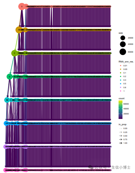
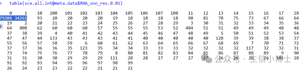
0.01分辨率下都有99个亚群，这个明显不合理。但是我们发现绝大部分细胞都在0和1群里

重新走一遍harmony整合流程

那我们把0和1群拿出来重新走一遍harmomy看看结果如何

    sce.all.int=sce.all.int[,sce.all.int@meta.data$RNA_snn_res.0.01 %in% c('0','1')];dim(sce.all.int)
    sce.all.int = run_harmony(sce.all.int)

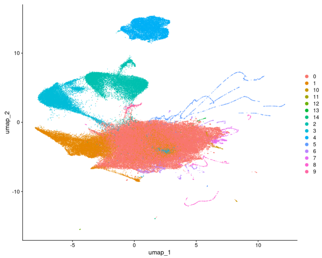
0.1分辨率还凑合

放大一点看看，看上去比原文干净了不少，但是有一些‘胡须’，值得深入研究一下

#####整合完成之后，查看0.1分辨率------
getwd();sp='human'
dir.create('check-by-0.1')
setwd('check-by-0.1')


sce.all.int@meta.data %>%head()
sel.clust = "RNA_snn_res.0.1"

sce.all.int <- SetIdent(sce.all.int, value = sel.clust)
table(sce.all.int@active.ident) 
print(getwd())

source('~/OLP_combine/scRNA_scripts/check-all-markers.R')
setwd('../') 
getwd()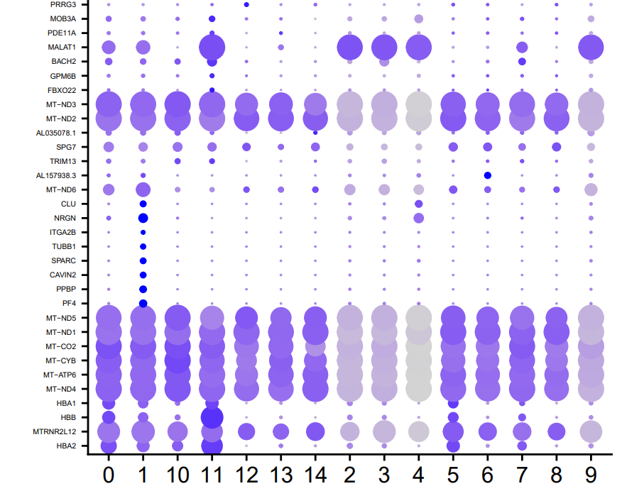

我们能够看到不管哪个亚群，线粒体基因都是挺高的

细胞注释

...

这里的细胞注释和前面一轮的细胞注释在技术上是一模一样的，我就不重复了

不足

存在的问题：

1. 作者共有4+16+13=33个样品，但是我这里只有七个GSM，说明作者把多个样本合并到一起去做了测序，这个信息在GSE201088_sampletag.csv.gz和GSE201088_sampleinfo.csv.gz文件里面应该是存在的。如果你想继续探索，可以把这两个文件中的信息加入seurat对象，继续下游分析。

2.原文作者说使用使用SCT v2进行了去除批次和normalize的操作，但是SCT v2不可以去除批次效应吧...(是我理解的不对吗)，作者使用0.4的分辨率得到了umap图。但是我使用harmony去除批次效应，0.01分辨率下竟然有99个亚群，但是0和1群占了绝大多数。所以后续我取了0和1群重新进行整合分析。最后，取0.1分辨率。

很多时候，我们都需要进行多轮的数据分析，直到最后的数据符合实际和实验设计。

3. BD的官方手册中提到细胞活力只要>50%就可以上机测序，这一点确实挺吸引人的。（比如有的课题组要做中性粒单细胞测序的话，估计会很喜欢50%这个数值。有研究报导中性粒在体外大约存活2-4h）但是这么低的活力就可能会导致本文中出现的情况：细胞死了很多，线粒体基因比例很高。

4.BD的中文教程确实少，BD想推广的话，不妨多搞一些教程和示例数据给大家分析分析。

5.由于第一次处理BD的数据，或许是我对本数据集的处理有问题，如有错误，请指教！

本文参与腾讯云自媒体分享计划，分享自微信公众号。

原始发表：2024-04-06，如有侵权请联系 cloudcommunity@tencent.com 删除

教程