单细胞数据分析|差异表达分析

单细胞数据分析|差异表达分析

在对单细胞数据进行差异表达分析的时候,可以从全细胞和元细胞两个角度去考虑。基于全细胞目前常见的单细胞转录组计算差异表达基因方法有DESeq2、edgeR、limma、MAST、SCDE (Single Cell Differential Expression)、Seurat (FindMarkers)、Monocle ( differentialGeneTest)、t-SNE/PCA-based methods。其中Seurat和DESeq2是医学研究中最常用的两种方法。基于元细胞的方法有SC3 (Single-Cell Consensus Clustering)、MetaCell。
下载地址:
https://figshare.com/ndownloader/files/34464122
01、数据预处理
首先读取数据:
import omicverse  as  ov
import  scanpy  as  sc
import  scvelo  as  scv
# 设置 Omicverse 绘图样式
ov.utils.ov_plot_set()
# 读取数据
adata = ov.read('data/kang.h5ad')
adata 
下面进行数据预处理。包括数据质量控制、标准化、选择高变基因(HVGs)并进行过滤。接着,代码对数据进行PCA降维,保留50个主成分,并进行非线性降维(MDE)。所有步骤旨在优化数据质量、减少噪声并提取重要的基因特征,为后续的分析(如聚类和差异表达分析)做准备。最终,处理后的数据存储在 adata 对象中。
# Quantity Control
adata = ov.pp.qc(adata, tresh={
    'mito_perc': 0.2,
    'nUMIs': 500,
    'detected_genes': 250
})
# Normalize and high variable genes (HVGs) calculated
adata = ov.pp.preprocess(adata, mode='shiftlog|pearson', n_HVGs=2000)
# Save the whole genes and filter the non-HVGs
adata.raw = adata
adata = adata[:, adata.var.highly_variable_features]
# Scale the adata.X
ov.pp.scale(adata)
# Dimensionality Reduction
ov.pp.pca(adata, layer='scaled', n_pcs=50)
# MDE and Embedding
adata.obsm['X_mde'] = ov.utils.mde(adata.obsm['scaled|original|X_pca'])
# Embedding Visualization
ov.utils.embedding(adata,
    basis='X_mde',
    frameon='small',
    color=['replicate', 'label', 'cell_type'])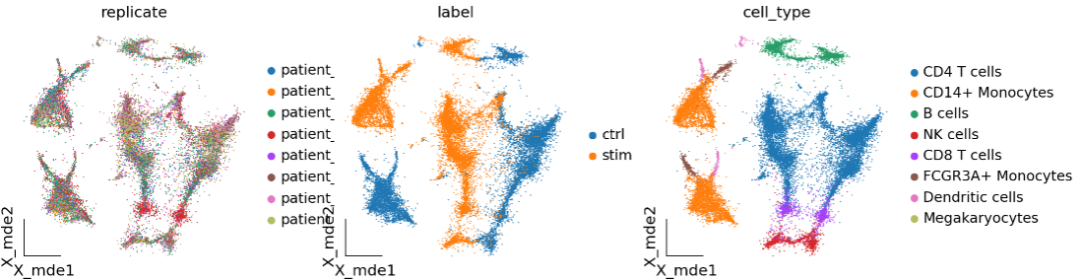
02、去批次 数据存在着一定的批次效应,这里使用Harmony进行批次效应的校正。
# 批次效应校正
adata_harmony = ov.single.batch_correction(adata, batch_key='replicate',
                                           methods='harmony', n_pcs=50)
# MDE计算
adata.obsm["X_mde_harmony"] = ov.utils.mde(adata.obsm["X_harmony"])

# 嵌入可视化
ov.utils.embedding(adata,
    basis='X_mde_harmony',
    frameon='small',
    color=['batch', 'cell_type'], show=False)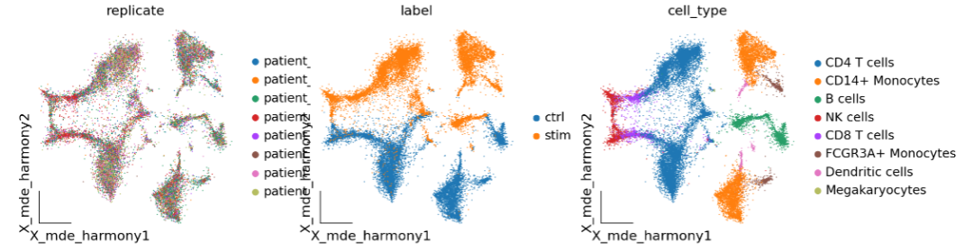
03、基于元细胞的差异表达分析
使用SEACells聚合细胞,然后在元细胞水平上,执行差异表达分析。值得一提的是,SEACells聚合的元细胞在信号聚合和细胞分辨率之间实现了最佳平衡,并且它们捕获整个表型谱中的细胞状态,包括罕见状态。元细胞保留了样本之间微妙的生物学差异,这些差异通过替代方法作为批次效应被消除,因此,为数据集成提供了比稀疏单个细胞更好的起点。
元细胞初始化
在这里,我们使用scaled|original|X_pca作为元细胞特征向量的初始化。
# Initialize MetaCell object
meta_obj = ov.single.MetaCell(adata, use_rep='scaled|original|X_pca', n_metacells=250,
    use_gpu=True)
# Initialize archetypes
meta_obj.initialize_archetypes()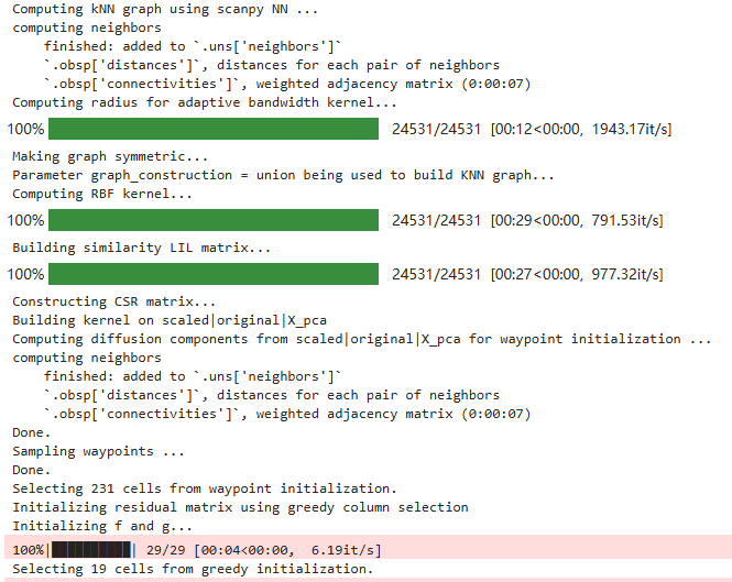
元细胞模型训练
初始完模型结构后,我们就需要对元细胞进行聚合,在这里我们通过训练SEACells模型来完成这一目的
# Train MetaCell model
meta_obj.train(min_iter=10, max_iter=50)
# Save the trained model
meta_obj.save('seacells/model.pkl')
# Load the trained model
meta_obj.load('seacells/model.pkl')
预测元细胞
可以使用 predicted 来预测原始 scRNA-seq 数据的元胞。有两种方法可供选择,一种是 "soft"方法,另一种是 "hard"方法。
# 创建新的细胞类型标签
meta_obj.adata.obs['celltype-label'] = [i + '-' + j for i, j in zip(meta_obj.adata.obs['cell_type'],
    meta_obj.adata.obs['label'])]

# 使用预测方法进行计算
ad = meta_obj.predicted(method='soft',
    celltype_label='celltype-label',
summarize_layer='lognorm')import matplotlib.pyplot as plt
# 创建绘图对象
fig, ax = plt.subplots(figsize=(4,4))
# 绘制嵌入图
ov.utils.embedding(meta_obj.adata,
basis='harmony',
color= ['cell_type'],
frameon='small',
title='Meta cells',
legend_fontsize=14,
legend_fontoutline=2,
size=10,
ax=ax,
alpha=0.2,
add_outline=False,
outline_color='black',
outline_width=1,
show=False)
# 绘制MetaCells
ov.single._metacell.plot_metacells(ax,meta_obj.adata,
use_rep='scaled|original|X_pca',
color='#CB3E35')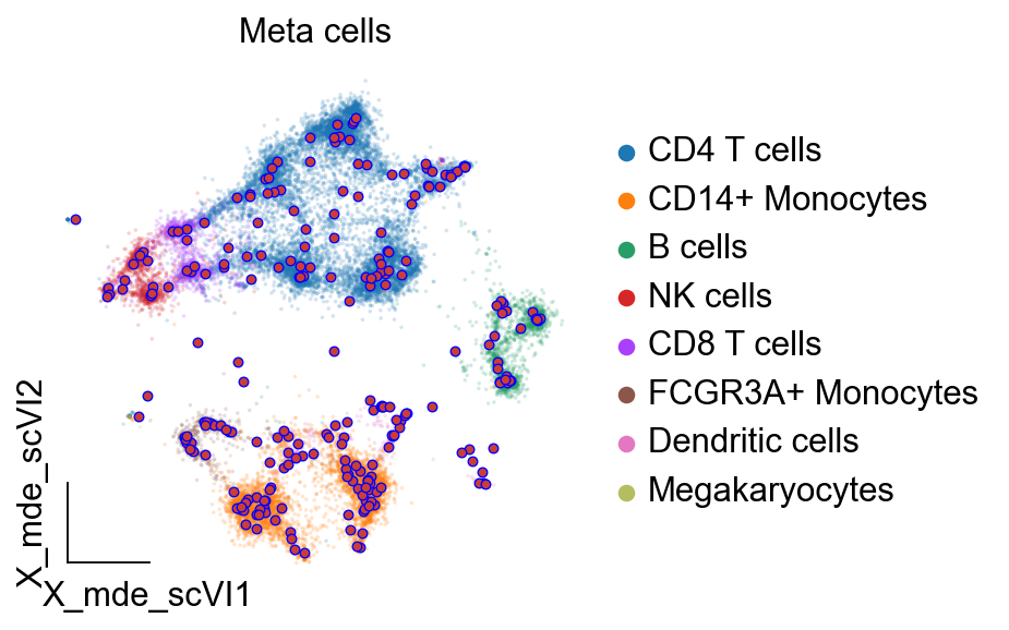
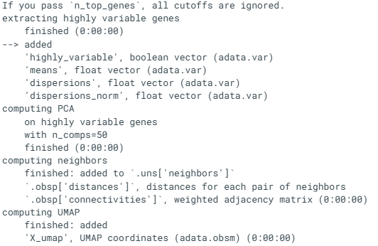
# 识别高变基因
sc.pp.highly_variable_genes(ad, n_top_genes=1500, inplace=True)
# 执行PCA降维
sc.tl.pca(ad, use_highly_variable=True)
# 计算邻近图
sc.pp.neighbors(ad, use_rep='X_pca')
# 执行UMAP可视化
sc.tl.umap(ad
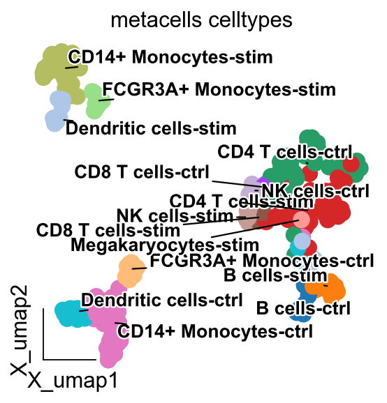
import  matplotlib.pyplot  as  plt
from  matplotlib  import  patheffects

# 创建绘图对象
fig, ax = plt.subplots(figsize=(4,4))

# 绘制嵌入图
ov.utils.embedding(ad,
    basis='X_umap',
    color= ['celltype'],
    frameon='small',
    title='metacells celltypes',
    legend_fontsize=14,
    legend_fontoutline=2,
    legend_loc=None,
    add_outline=False,
    outline_color='black',
    outline_width=1,
    show=False)

# 绘制细胞类型标签
ov.utils.gen_mpl_labels(ad,
    'celltype',
    exclude=("None",),
    basis='X_umap',
    ax=ax,
    adjust_kwargs=dict(arrowprops=dict('arrowstyle'='-', 'color'='black')),
    text_kwargs=dict(fontsize=12, weight='bold',
    path_effects=[patheffects.withStroke(linewidth=2, foreground='w')] )
# 选择细胞类型并过滤数据
test_adata = ad[ad.obs['celltype'].isin(['CD4 T cells-stim', 'CD4 T cells-ctrl'])]

# 执行差异表达分析
dds_meta = ov.bulk.pyDEG(test_adata.to_df().T)
dds_meta.drop_duplicates_index()
print('... drop_duplicates_index success')
# 获取处理组和对照组的样本
treatment_groups = test_adata.obs[test_adata.obs['celltype'] == 'CD4 T cells-stim'].index.tolist()
control_groups = test_adata.obs[test_adata.obs['celltype'] == 'CD4 T cells-ctrl'].index.tolist()
# 进行差异表达分析
dds_meta.deg_analysis(treatment_groups, control_groups, method='ttest')

# 设置foldchange和p值阈值
dds_meta.foldchange_set(fc_threshold=-1, pval_threshold=0.05, logp_max=10)
# 绘制火山图
dds_meta.plot_volcano(title='DEG Analysis', figsize=(4, 4), plot_genes_num=8, plot_genes_fontsize=12)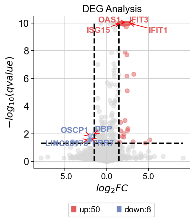
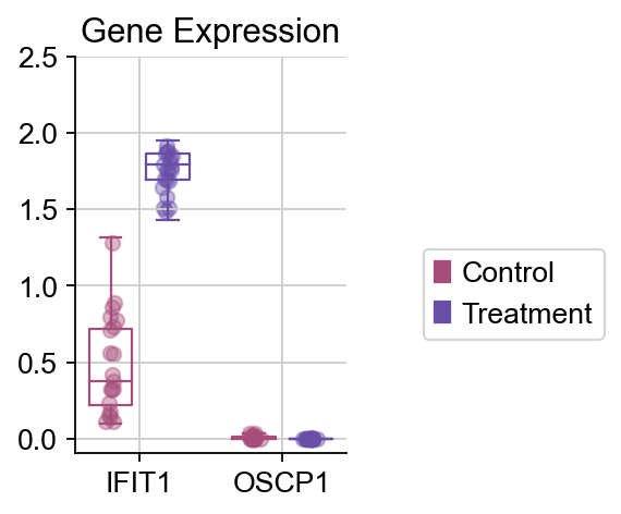
# 绘制基因表达的箱型图
dds_meta.plot_boxplot(genes= ['IFIT1', 'OSCP1'],
    treatment_groups=treatment_groups,
    control_groups=control_groups,
    figsize=(2,3),
    fontsize=12,
    legend_bbox=(2, 0.55))
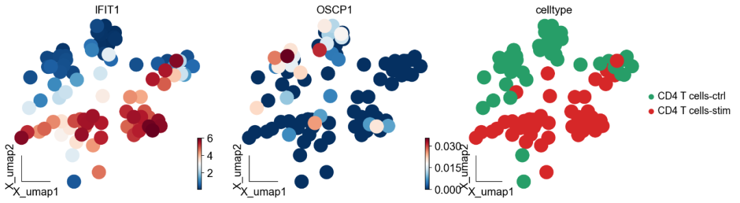
# 绘制UMAP嵌入图
ov.utils.embedding(test_adata,
    basis='X_umap',
    frameon='small',
    color= ['IFIT1', 'OSCP1', 'celltype'],
    cmap='RdBu_r')
# 绘制嵌入图
ov.utils.embedding(adata,
    basis='harmony',
    frameon='small',
    color= ['label', 'IFIT1', 'OSCP1'])
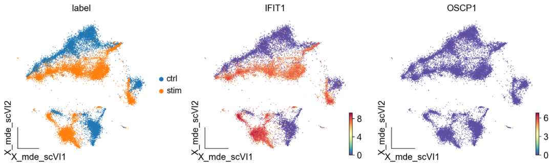
可以发现,IFIT1和OSCP1分别在stim和ctrl组中特异性下调与上调,其中IFIT1编码一种含有四肽重复序列的蛋白质,最初被鉴定为干扰素治疗诱导的。元细胞显示出了更优的差异基因的识别优势,并且排除了dropout的干扰。
总结: 本节我们选择元细胞作为分析策略避免生物学噪音和dropout的干扰。
腾讯云开发者
