03-使用PyTorch处理最简单的神经网络分类任务(笔记+代码)

03-使用PyTorch处理最简单的神经网络分类任务(笔记+代码)

本文为PyTorch Neural Network Classification[1](https://www.learnpytorch.io)的学习笔记,对原文进行了翻译和编辑,本系列课程介绍和目录在《使用PyTorch进行深度学习系列》课程介绍[2]。 文章将最先在我的博客[3]发布,其他平台因为限制不能实时修改。 在微信公众号内无法嵌入超链接,可以点击底部阅读原文[4]获得更好的阅读体验。
目录:
0.分类神经网络的架构:
- 1. 制作分类数据
- 1.1 输入和输出形状
- 1.2 将数据转换为张量并创建训练和测试分割
- 2. 建立模型
- 2.2定义损失函数和优化器
- 3. 训练模型
- 3.1从原始模型输出到预测标签
- 3.2 正式训练和测试模型
- 4. 进行预测并评估模型
- 5. 改进模型(从模型角度)
- 6.非线性模型
- 6.1 定义非线性模型
- 6.2 训练非线性模型
- 7 在PyTorch中构建多类分类模型
- 7.1创建数据集
- 7.2 创建模型
- 7.3 创建损失函数和优化器
- 7.4 正式训练
- 7.5 进行预测和评估
- 8.更多分类评估指标
- 感谢
分类和回归是最常见的机器学习问题类型之一。在本笔记中,我们将使用 PyTorch 解决几个不同的分类问题(二元分类,多类分类,多标签分类)。换句话说,我们通过获取一组输入并预测这些输入集属于哪个类别。
下列图示了三种分类情况:
- 二元分类 Binary classification
- 多类分类 Multi-class classification
- 多标签分类 Multi-label classification
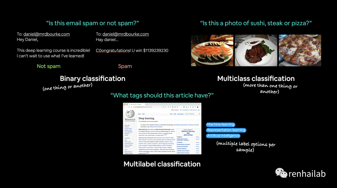
三种分类情况介绍
0.分类神经网络的架构:
结合 深度学习之神经网络的结构的视频(强烈建议观看)[5],识别手写数字0-9的神经网络可以简化为下图:
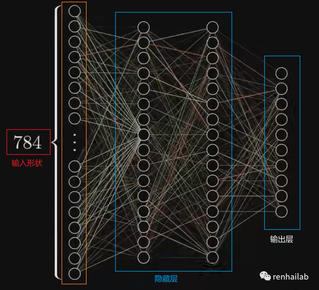
详细来说,分类神经网络的架构总结如下表,后面会单独解释:
超参数 | 二元分类 | 多类分类 |
|---|---|---|
输入层形状 (in_features) | 与特征数量相同(例如,心脏病预测中的年龄、性别、身高、体重、吸烟状况,输入层为 5个) | 同左 |
隐藏层(Hidden layer(s)) | 至少有一个1 | 同左 |
每个隐藏层的神经元(Neurons per hidden layer) | 一般为 10 到 512 | 同左 |
输出层形状 (out_features) | 一个或多个类别 | 每班 1 张(例如食物、人或狗照片 3 张) |
隐藏层激活(Hidden layer activation) | 通常是 ReLU[6](修正线性单元),但也可以是许多其他单元 | |
输出激活(Output activation) | Sigmoid(PyTorch 中的 torch.sigmoid[7] ) | Softmax(PyTorch 中的 torch.softmax[8] ) |
损失函数(Loss function) | 二元交叉熵(PyTorch 中的 torch.nn.BCELoss ) | 交叉熵(PyTorch 中的 torch.nn.CrossEntropyLoss[9] ) |
优化器(Optimizer ) | SGD[10](随机梯度下降),Adam[11](有关更多选项,请参阅 torch.optim[12] ) | 同左 |
1. 制作分类数据
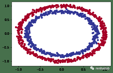
我们将使用 Scikit-Learn 中的 `make_circles()`[13] 方法生成两个具有不同颜色点的圆圈。
from sklearn.datasets import make_circles


# Make 1000 samples
n_samples = 1000

# Create circles
X, y = make_circles(n_samples,
                    noise=0.03, # a little bit of noise to the dots
                    random_state=42) # keep random state so we get the same values
查看前 5 个 X 和 y 值。
print(f"First 5 X features:\n{X[:5]}")
print(f"\nFirst 5 y labels:\n{y[:5]}")
>>>
First 5 X features:
[[ 0.75424625  0.23148074]
 [-0.75615888  0.15325888]
 [-0.81539193  0.17328203]
 [-0.39373073  0.69288277]
 [ 0.44220765 -0.89672343]]

First 5 y labels:
[1 1 1 1 0]
看起来每个 y 值有两个 X 值。
绘制出来:
# 转换为pandas的Dataframe对象
import pandas as pd
import matplotlib.pyplot as plt

circles = pd.DataFrame({"X1": X[:, 0],
    "X2": X[:, 1],
    "label": y
})
circles.head(10)

# 可视化
plt.scatter(x=X[:, 0],
            y=X[:, 1],
            c=y,
            cmap=plt.cm.RdYlBu);
circles
1.1 输入和输出形状
深度学习中最常见的错误之一是形状错误。张量和张量运算的形状不匹配会导致模型出现错误。
我们查看circles的形状:
# Check the shapes of our features and labels
X.shape, y.shape
>>>
((1000, 2), (1000,))
有 1000 个 X 和 1000 个 y 。分别X和y查看第一个数据:
# View the first example of features and labels
X_sample = X[0]
y_sample = y[0]
print(f"Values for one sample of X: {X_sample} and the same for y: {y_sample}")
print(f"Shapes for one sample of X: {X_sample.shape} and the same for y: {y_sample.shape}")
>>>
Values for one sample of X: [0.75424625 0.23148074] and the same for y: 1
Shapes for one sample of X: (2,) and the same for y: ()
可以看到X即代表点的坐标,y即代表类别,两个输入特征对应一个输出特征。
1.2 将数据转换为张量并创建训练和测试分割
具体分为:
- 将我们的数据转换为张量(现在我们的数据位于 NumPy 数组中,而 PyTorch 更喜欢使用 PyTorch 张量)。
- 将我们的数据分为训练集和测试集(我们将在训练集上训练模型以学习
X和y之间的模式,然后在测试数据集上评估这些学习到的模式) 。
# 将数据转换为张量

import torch
X = torch.from_numpy(X).type(torch.float)
y = torch.from_numpy(y).type(torch.float)

#查看前五条数据
X[:5], y[:5]

>>>
(tensor([[ 0.7542,  0.2315],
         [-0.7562,  0.1533],
         [-0.8154,  0.1733],
         [-0.3937,  0.6929],
         [ 0.4422, -0.8967]]),
 tensor([1., 1., 1., 1., 0.]))
现在我们的数据是张量格式,让我们将其分为训练集和测试集。
此处不用手动分割,我们使用 Scikit-Learn 中有用的函数 `train_test_split()`[14] 。
# 分为训练集和测试集
from sklearn.model_selection import train_test_split

X_train, X_test, y_train, y_test = train_test_split(X,
                                                    y,
                                                    test_size=0.2, # 80% 训练,20% 测试
                                                    random_state=42) # 固定seed 可重现

len(X_train), len(X_test), len(y_train), len(y_test)
>>>
(800, 200, 800, 200)
我们现在有 800 个训练样本和 200 个测试样本。
2. 建立模型
(1)通过子类化 nn.Module 自定义模型
import torch
from torch import nn

# 设置device
device = "cuda" if torch.cuda.is_available() else "cpu"

# 1. 继承 nn.Module
class CircleModelV0(nn.Module):
    def __init__(self):
        super().__init__()
        # 2.创建两个线性层
        self.layer_1 = nn.Linear(in_features=2, out_features=5) # 输入 2 features (X), 输出 5 features
        self.layer_2 = nn.Linear(in_features=5, out_features=1) # 输入 5 features, 输出 1 feature (y)

    # 3.定义一个包含模型前向传递计算的 forward() 方法。
    def forward(self, x):
        return self.layer_2(self.layer_1(x))

# 4.实例化模型并将其发送到目标device
model_0 = CircleModelV0().to(device)
model_0
self.layer_1 采用 2 个输入特征 in_features=2 并生成 5 个输出特征 out_features=5 。这被称为具有 5 个隐藏单元或神经元。该层将输入数据从 2 个特征变成 5 个特征。这使得模型能够从 5 个数字而不是 2 个数字中学习模式,从而可能产生更好的输出。
隐藏单元的唯一规则是下一层(在我们的例子中) self.layer_2 必须采用与上一层 out_features 相同的 in_features 。

A visual example of what a classification neural network with linear activation looks like on the tensorflow playground
与我们刚刚构建的分类神经网络类似的分类神经网络的直观示例。尝试在 TensorFlow Playground[15] 网站上创建您自己的一个。
(2)利用nn.Sequential
nn.Sequential 按照输入数据出现的顺序对各层执行前向传递计算。您还可以使用 nn.Sequential 执行与上面相同的操作:
model_0 = nn.Sequential(
    nn.Linear(in_features=2, out_features=5),
    nn.Linear(in_features=5, out_features=1)
).to(device)

model_0
Sequential(
  (0): Linear(in_features=2, out_features=5, bias=True)
  (1): Linear(in_features=5, out_features=1, bias=True)
)
nn.Sequential 对于直接计算来说非常棒,但是,正如命名空间所说,它总是按顺序运行。
(3)测试模型
让我们看看当我们通过它传递一些数据时会发生什么。
# 用模型预测
untrained_preds = model_0(X_test.to(device))
print(f"预测结果的长度: {len(untrained_preds)}, Shape: {untrained_preds.shape}")
print(f"测试样本的长度: {len(y_test)}, Shape: {y_test.shape}")
print(f"\n前十行预测结果:\n{untrained_preds[:10]}")
print(f"\n前十行测试标签:\n{y_test[:10]}")
输出:
预测结果的长度:  200, Shape: torch.Size([200, 1])
测试样本的长度:  200, Shape: torch.Size([200])

前十行预测结果:
tensor([[-0.4279],
        [-0.3417],
        [-0.5975],
        [-0.3801],
        [-0.5078],
        [-0.4559],
        [-0.2842],
        [-0.3107],
        [-0.6010],
        [-0.3350]], device='cuda:0', grad_fn=<SliceBackward0>)

前十行测试标签:
tensor([1., 0., 1., 0., 1., 1., 0., 0., 1., 0.])
看起来预测的数量与测试标签的数量相同,但预测结果(非0或1)看起来与测试标签(0或者1)的形式或形状不同。之后我们会解决这个问题。
2.2定义损失函数和优化器
我们需要一个损失函数来度量预测的效果。 不同的问题类型需要不同的损失函数。例如,对于回归问题(预测数字),您可能会使用平均绝对误差 (MAE) 损失。对于二元分类问题(例如我们的问题),您通常会使用二元交叉熵作为损失函数。
交叉熵损失:所有标签分布与预期间的损失值。
然而,相同的优化器函数通常可以在不同的问题空间中使用。例如,随机梯度下降优化器(SGD, torch.optim.SGD() )可用于解决一系列问题,这同样适用于 Adam 优化器( torch.optim.Adam() )。
Loss function/Optimizer 损失函数/优化器 | Problem type 问题类型 | PyTorch Code PyTorch 代码 |
|---|---|---|
Stochastic Gradient Descent (SGD) optimizer 随机梯度下降 (SGD) 优化器 | Classification, regression, many others. 分类、回归等等。 | `torch.optim.SGD()`[16] |
Adam Optimizer 亚当优化器 | Classification, regression, many others. 分类、回归等等。 | `torch.optim.Adam()`[17] |
Binary cross entropy loss 二元交叉熵损失 | Binary classification 二元分类 | `torch.nn.BCELossWithLogits`[18] or `torch.nn.BCELoss`[19] torch.nn.BCELossWithLogits 或 torch.nn.BCELoss |
Cross entropy loss 交叉熵损失 | Mutli-class classification 多类分类 | `torch.nn.CrossEntropyLoss`[20] |
Mean absolute error (MAE) or L1 Loss 平均绝对误差 (MAE) 或 L1 损失 | Regression 回归 | `torch.nn.L1Loss`[21] |
Mean squared error (MSE) or L2 Loss 均方误差 (MSE) 或 L2 损失 | Regression 回归 | `torch.nn.MSELoss`[22] |
由于我们正在处理二元分类问题,因此我们使用二元交叉熵损失函数。
注意:回想一下,损失函数用于衡量模型预测的错误程度,损失越高,模型越差。
PyTorch 有两种二元交叉熵实现:
- `torch.nn.BCELoss()`[23] - 创建一个损失函数,用于测量目标(标签)和输入(特征)之间的二元交叉熵。
- `torch.nn.BCEWithLogitsLoss()`[24] - 这与上面相同,只是它有一个内置的 sigmoid 层 (
nn.Sigmoid)。
应该使用哪一个?
`torch.nn.BCEWithLogitsLoss()` 的文档[25]指出,它比在 nn.Sigmoid 层之后使用 torch.nn.BCELoss() 更稳定。所以一般来说,torch.nn.BCEWithLogitsLoss() 是更好的选择。
让我们创建一个损失函数和一个优化器。
对于优化器,我们将使用 torch.optim.SGD() 以学习率 0.1 优化模型参数。
# 创建一个损失函数
loss_fn = nn.BCEWithLogitsLoss()

# 创建一个优化器
optimizer = torch.optim.SGD(params=model_0.parameters(),
                            lr=0.1)
现在我们还创建一个评估指标。
评估指标可用于提供有关模型进展情况的另一个视角。有多种评估指标可用于分类问题,但让我们从准确性accuracy开始。
准确度可以通过将正确预测总数除以预测总数来衡量。例如,如果模型能够在 100 次预测中做出 99 次正确的预测,则准确率将达到 99%。
编写一个函数来执行此操作。
# 计算 准确性  (a classification metric)
def accuracy_fn(y_true, y_pred):
    # 1.torch.eq() 用于逐元素地比较两个张量的相等性。它返回一个新的布尔张量,其中每个元素都表示对应位置上的元素是否相等。
    # 2.使用 .sum() 方法对布尔张量进行求和操作,将所有为 True 的元素加起来。
    # 3.使用 .item() 方法将结果转换为 Python 的标量值。
    correct = torch.eq(y_true, y_pred).sum().item()
    acc = (correct / len(y_pred)) * 100
    return acc
3. 训练模型
在PyTorch工作流程基础知识【PyTorch 深度学习系列】[26]中,我们已经学习了训练模型的基本步骤,不记得的可以回顾一下(提示:前向传递-计算损失-归零梯度-对损失执行反向传播-梯度下降)。
3.1从原始模型输出到预测标签
对模型预测之后,我们需要将预测的输出值对应到相应的特征,我们先看看模型在向前传递之后,输出的值是什么样子的:
为此,我们向模型传递一些数据。
# 查看针对测试数据的预测值的前五项
y_logits = model_0(X_test.to(device))[:5]
y_logits
tensor([[-0.4279],
        [-0.3417],
        [-0.5975],
        [-0.3801],
        [-0.5078]], device='cuda:0', grad_fn=<SliceBackward0>)
y_logits代表的数字很难理解,我们需要它能代表我们真实的标签(此处是0或者1),即通过logits -> 预测概率 -> 预测标签的流程,将原始输出转化为真实的标签:
(logits -> 预测概率 -> 预测标签):logits -> prediction probabilities -> prediction labels的过程
logits -> prediction probabilities -> prediction labels的过程
forward()方程的未修改的原始输出( y )以及我们模型的原始输出通常称为 logits。
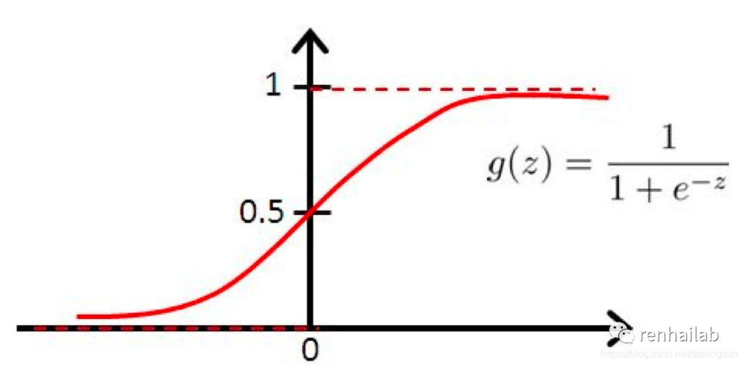
为了将模型的原始输出(logits)转换为标签,我们可以使用 **sigmoid 激活函数**[27],将输入实数值并将其“挤压”到0到1范围内。
在代码中这样实现:
y_pred_probs = torch.sigmoid(y_logits)
y_pred_probs
>>>
tensor([[0.3946],
        [0.4154],
        [0.3549],
        [0.4061],
        [0.3757]], device='cuda:0', grad_fn=<SigmoidBackward0>)
数值被压缩到0到1,在二分类问题上,趋近于0和趋近于1的数值被分为两类,越接近0,模型越认为样本属于0类,越接近1,模型越认为样本属于1类。他们之间的界限则为0.5,我们可以通过取整(四舍五入)来实现分类。
更确切的说:
- 如果
y_pred_probs>= 0.5,则y=1(1 类) - 如果
y_pred_probs< 0.5,y=0(0 级)
在代码中:
# 对结果取整(round)
y_preds = torch.round(y_pred_probs)

# 整个logits -> prediction probabilities -> prediction labels的过程的过程:
y_pred_labels = torch.round(torch.sigmoid(model_0(X_test.to(device))[:5]))

# 逐一检查两个tensor是否相等
print(torch.eq(y_preds.squeeze(), y_pred_labels.squeeze()))

# 删除多余维度
y_preds.squeeze()
输出:
tensor([True, True, True, True, True], device='cuda:0')
tensor([0., 0., 0., 0., 0.], device='cuda:0', grad_fn=<SqueezeBackward0>)
把我们预测的标签和真实的标签y_test对比:
y_test[:5]
>>>
tensor([1., 0., 1., 0., 1.])
和y_preds:tensor([0., 0., 0., 0., 0.])对比,有对有错。
sigmoid 激活函数的使用通常仅适用于二元分类 logits。对于多类分类,我们将考虑使用 softmax 激活函数[28](稍后会介绍)。
当将模型的原始输出传递给 nn.BCEWithLogitsLoss 时,不需要使用 sigmoid 激活函数(logits 损失中的“logits”是因为它作用于模型的原始 logits 输出),这是因为它内置 sigmoid 函数。
3.2 正式训练和测试模型
首先训练 100 个 epoch,并每 10 个 epoch 输出模型的进度。
torch.manual_seed(42)

# 设置迭代次数
epochs = 100

# 将数据传输到device(前文定义过)
X_train, y_train = X_train.to(device), y_train.to(device)
X_test, y_test = X_test.to(device), y_test.to(device)

# 进行训练和评估循环
for epoch in range(epochs):
    ### 训练
    model_0.train()

    # 1. 向前传播
    y_logits = model_0(X_train).squeeze() # squeeze to remove extra `1` dimensions,
    y_pred = torch.round(torch.sigmoid(y_logits)) # turn logits -> pred probs -> pred labls

    # 2. 计算损失和准确度
    loss = loss_fn(y_logits, # 使用前文定义的nn.BCEWithLogitsLoss二元交叉熵损失
                   y_train)
    acc = accuracy_fn(y_true=y_train,
                      y_pred=y_pred)

    # 3. 归零梯度
    optimizer.zero_grad()

    # 4.通过进行反向传播来计算梯度
    loss.backward()

    # 5. 过调用优化器来更新模型参数
    optimizer.step()

    ### 测试
    model_0.eval()
    with torch.inference_mode():
        # 1. 向前传播
        test_logits = model_0(X_test).squeeze()
        test_pred = torch.round(torch.sigmoid(test_logits))
        # 2. 计算损失
        test_loss = loss_fn(test_logits,
                            y_test)
        test_acc = accuracy_fn(y_true=y_test,
                               y_pred=test_pred)

    # 10个循环输出一次结果
    if epoch % 10 == 0:
        print(f"Epoch: {epoch} | Loss: {loss:.5f}, Accuracy: {acc:.2f}% | Test loss: {test_loss:.5f}, Test acc: {test_acc:.2f}%")
Epoch: 0 | Loss: 0.72090, Accuracy: 50.00% | Test loss: 0.72196, Test acc: 50.00%
Epoch: 10 | Loss: 0.70291, Accuracy: 50.00% | Test loss: 0.70542, Test acc: 50.00%
Epoch: 20 | Loss: 0.69659, Accuracy: 50.00% | Test loss: 0.69942, Test acc: 50.00%
Epoch: 30 | Loss: 0.69432, Accuracy: 43.25% | Test loss: 0.69714, Test acc: 41.00%
Epoch: 40 | Loss: 0.69349, Accuracy: 47.00% | Test loss: 0.69623, Test acc: 46.50%
Epoch: 50 | Loss: 0.69319, Accuracy: 49.00% | Test loss: 0.69583, Test acc: 46.00%
Epoch: 60 | Loss: 0.69308, Accuracy: 50.12% | Test loss: 0.69563, Test acc: 46.50%
Epoch: 70 | Loss: 0.69303, Accuracy: 50.38% | Test loss: 0.69551, Test acc: 46.00%
Epoch: 80 | Loss: 0.69302, Accuracy: 51.00% | Test loss: 0.69543, Test acc: 46.00%
Epoch: 90 | Loss: 0.69301, Accuracy: 51.00% | Test loss: 0.69537, Test acc: 46.00%
每次数据分割的准确率几乎没有超过 50%,效果不理想。我们将我们的结果绘制出来:
4. 进行预测并评估模型
让我们画出模型的预测,为此我们需要下载 Learn PyTorch for Deep Learning 存储库[29]中的`helper_functions.py`[30] 脚本,它包含一个名为 plot_decision_boundary() 的有用函数,它创建一个 NumPy 网格来直观地绘制我们的模型预测某些类的不同点。
我们还将导入我们在笔记本 01 中编写的 plot_predictions() 以供稍后使用。
import requests
from pathlib import Path

# Download helper functions from Learn PyTorch repo (if not already downloaded)
if Path("helper_functions.py").is_file():
  print("helper_functions.py already exists, skipping download")
else:
  print("Downloading helper_functions.py")
  request = requests.get("https://raw.githubusercontent.com/mrdbourke/pytorch-deep-learning/main/helper_functions.py")
  with open("helper_functions.py", "wb") as f:
    f.write(request.content)

from helper_functions import plot_predictions, plot_decision_boundary
绘图:
# 绘制训练和测试数据的边界
plt.figure(figsize=(12, 6))
plt.subplot(1, 2, 1)
plt.title("Train")
plot_decision_boundary(model_0, X_train, y_train)
plt.subplot(1, 2, 2)
plt.title("Test")
plot_decision_boundary(model_0, X_test, y_test)

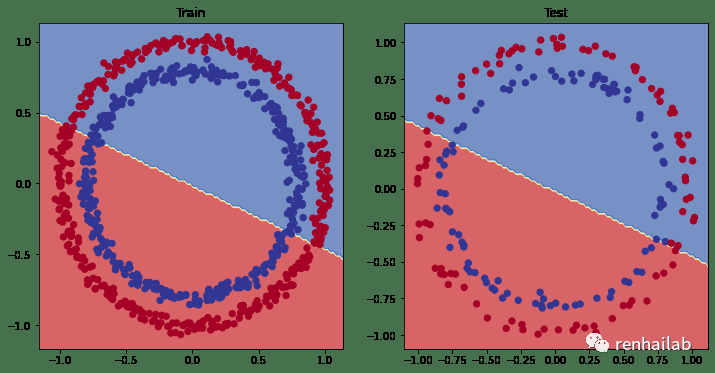
训练(左)和测试(右)数据的边界
很明显,我们正在使用直线来分割红点和蓝点,由于我们的数据是圆形的,画一条直线最多只能将其从中间切掉。所以基本模型只能有50% 的准确率。
用机器学习术语来说,我们的模型欠拟合,它没有从数据中学习预测模式。
我们如何改进这一点?
5. 改进模型(从模型角度)
让我们尝试解决模型的欠拟合问题。
特别关注模型(而不是数据),我们可以通过几种方法来做到这一点。
模型改进技术 | 它有什么作用? |
|---|---|
添加更多层 | 每一层都可能增加模型的学习能力,每层都能够学习数据中的某种新模式,更多层通常被称为使神经网络更深。 |
添加更多隐藏单位 | 与上面类似,每层更多的隐藏单元意味着模型学习能力的潜在增加,更多的隐藏单元通常被称为使你的神经网络更宽。 |
训练更多此more epochs | 如果您的模型有更多机会查看数据,它可能会了解更多信息。 |
更改激活函数 | 有些数据不能只用直线拟合(就像我们所看到的那样),使用非线性激活函数可以帮助解决这个问题。 |
改变学习率 | 模型特定性较少,但仍然相关,优化器的学习率决定模型每一步应改变其参数的程度,太多,模型会过度校正,太少,则学习得不够。 |
改变损失函数 | 同样,虽然模型不太具体,但仍然很重要,不同的问题需要不同的损失函数。例如,二元交叉熵损失函数不适用于多类分类问题。 |
使用迁移学习 | 从与您的问题域类似的问题域中获取预训练模型,并将其调整为您自己的问题。我们在06-PyTorch迁移学习:在预训练模型上进行训练[31]中介绍了迁移学习。 |
原文[32]中进行了第一次改进:在模型添加一个额外的层,增加训练 次数( epochs=1000 )并在将隐藏层中神经元的数量增加到10个,结果如下图:
第一次改进后的训练测试可视化结果
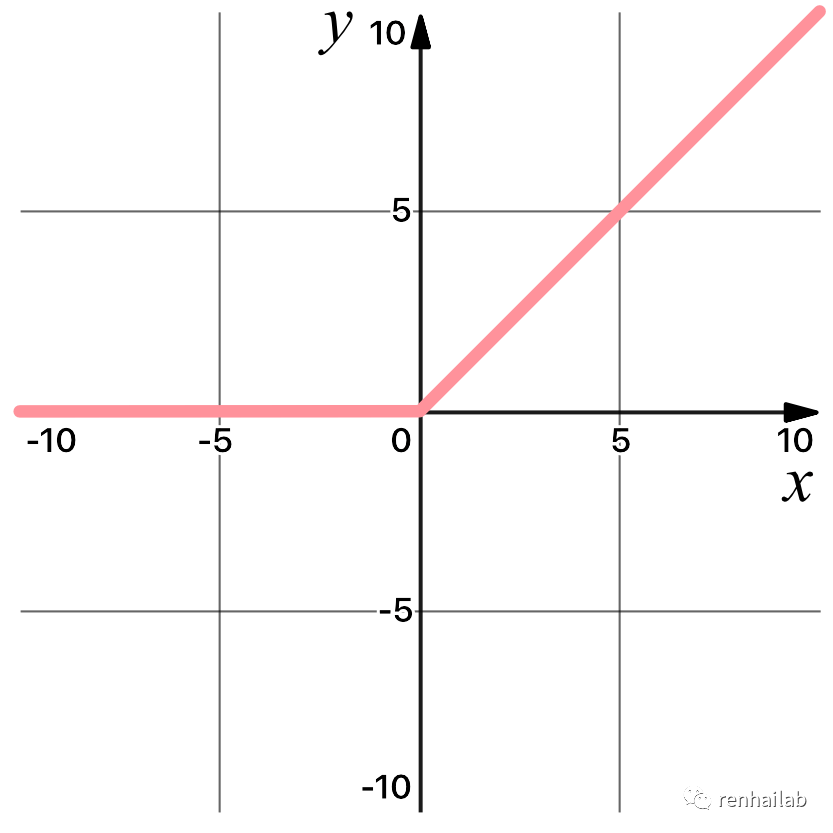
模型仍然在红点和蓝点之间画一条直线。显然不符合我们的需求,正确的方法是进行非线性建模,并且引入非线性激活函数。PyTorch 有个一堆现成的非线性激活函数[33],最常见和性能最好的之一是 **[ReLU](https://en.wikipedia.org/wiki/Rectifier_(neural_networks "ReLU")**(修正线性单元, `torch.nn.ReLU()`[34] )。
ReLU激活函数是一对一的数学运算,该激活函数按元素应用于输入张量中的每个值。例如,如果对值 2.24 应用 ReLU,结果将为 2.24,因为 2.24 大于 0。:
现在不理解不要紧,我们在后面会多次提到ReLU激活函数。
6.非线性模型
6.1 定义非线性模型
我们利用ReLU激活函数,重新定义一个非线性模型:
from torch import nn
class CircleModelV2(nn.Module):
    def __init__(self):
        super().__init__()
        self.layer_1 = nn.Linear(in_features=2, out_features=10)
        self.layer_2 = nn.Linear(in_features=10, out_features=10)
        self.layer_3 = nn.Linear(in_features=10, out_features=1)
        self.relu = nn.ReLU() # <- add in ReLU activation function

    def forward(self, x):
       return self.layer_3(self.relu(self.layer_2(self.relu(self.layer_1(x)))))

model_3 = CircleModelV2().to(device)
print(model_3)
CircleModelV2(
  (layer_1): Linear(in_features=2, out_features=10, bias=True)
  (layer_2): Linear(in_features=10, out_features=10, bias=True)
  (layer_3): Linear(in_features=10, out_features=1, bias=True)
  (relu): ReLU()
)
6.2 训练非线性模型
torch.manual_seed(42)

# 设置迭代次数
epochs = 100

# 将数据传输到device(前文定义过)
X_train, y_train = X_train.to(device), y_train.to(device)
X_test, y_test = X_test.to(device), y_test.to(device)

# 进行训练和评估循环
for epoch in range(epochs):
    ### 训练
    model_0.train()

    # 1. 向前传播
    y_logits = model_3(X_train).squeeze() # squeeze to remove extra `1` dimensions,
    y_pred = torch.round(torch.sigmoid(y_logits)) # turn logits -> pred probs -> pred labls

    # 2. 计算损失和准确度
    loss = loss_fn(y_logits, # 使用前文定义的nn.BCEWithLogitsLoss二元交叉熵损失
                   y_train)
    acc = accuracy_fn(y_true=y_train,
                      y_pred=y_pred)

    # 3. 归零梯度
    optimizer.zero_grad()

    # 4.通过进行反向传播来计算梯度
    loss.backward()

    # 5. 过调用优化器来更新模型参数
    optimizer.step()

    ### 测试
    model_0.eval()
    with torch.inference_mode():
        # 1. 向前传播
        test_logits = model_3(X_test).squeeze()
        test_pred = torch.round(torch.sigmoid(test_logits))
        # 2. 计算损失
        test_loss = loss_fn(test_logits,
                            y_test)
        test_acc = accuracy_fn(y_true=y_test,
                               y_pred=test_pred)

    # 10个循环输出一次结果
    if epoch % 10 == 0:
        print(f"Epoch: {epoch} | Loss: {loss:.5f}, Accuracy: {acc:.2f}% | Test loss: {test_loss:.5f}, Test acc: {test_acc:.2f}%")
Epoch: 0 | Loss: 0.69295, Accuracy: 50.00% | Test Loss: 0.69319, Test Accuracy: 50.00%
Epoch: 100 | Loss: 0.69115, Accuracy: 52.88% | Test Loss: 0.69102, Test Accuracy: 52.50%
Epoch: 200 | Loss: 0.68977, Accuracy: 53.37% | Test Loss: 0.68940, Test Accuracy: 55.00%
Epoch: 300 | Loss: 0.68795, Accuracy: 53.00% | Test Loss: 0.68723, Test Accuracy: 56.00%
Epoch: 400 | Loss: 0.68517, Accuracy: 52.75% | Test Loss: 0.68411, Test Accuracy: 56.50%
Epoch: 500 | Loss: 0.68102, Accuracy: 52.75% | Test Loss: 0.67941, Test Accuracy: 56.50%
Epoch: 600 | Loss: 0.67515, Accuracy: 54.50% | Test Loss: 0.67285, Test Accuracy: 56.00%
Epoch: 700 | Loss: 0.66659, Accuracy: 58.38% | Test Loss: 0.66322, Test Accuracy: 59.00%
Epoch: 800 | Loss: 0.65160, Accuracy: 64.00% | Test Loss: 0.64757, Test Accuracy: 67.50%
Epoch: 900 | Loss: 0.62362, Accuracy: 74.00% | Test Loss: 0.62145, Test Accuracy: 79.00%
看起来好多了!
绘制出来:
# Make predictions
model_3.eval()
with torch.inference_mode():
    y_preds = torch.round(torch.sigmoid(model_3(X_test))).squeeze()
y_preds[:10], y[:10] # want preds in same format as truth labels
(tensor([1., 0., 1., 0., 0., 1., 0., 0., 1., 0.], device='cuda:0'),
 tensor([1., 1., 1., 1., 0., 1., 1., 1., 1., 0.]))
# Plot decision boundaries for training and test sets
plt.figure(figsize=(12, 6))
plt.subplot(1, 2, 1)
plt.title("Train")
plot_decision_boundary(model_1, X_train, y_train) # model_1 = no non-linearity
plt.subplot(1, 2, 2)
plt.title("Test")
plot_decision_boundary(model_3, X_test, y_test) # model_3 = has non-linearity
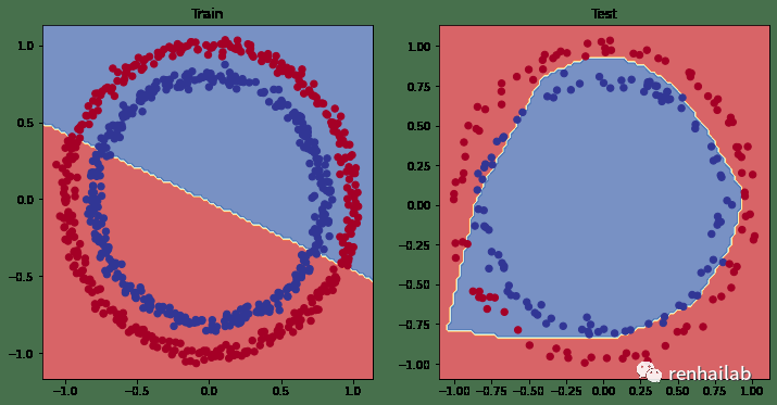
使用非线性模型训练和测试结果可视化
7 在PyTorch中构建多类分类模型
二元分类问题涉及将某些内容分类为两个选项之一(例如,将一张照片分类为猫照片或狗照片),而多类分类问题则涉及从两个以上选项的列表中对某些内容进行分类(例如,分类)猫、狗或鸡的照片)。
总所周知的ImageNet-1k[35] 数据集,有 1000 个输出类。
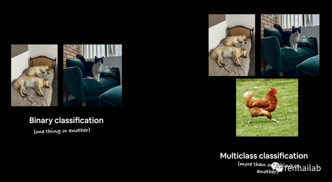
二元分类与多类分类的示例
7.1创建数据集
使用`sklearn.datasets`[36]模块中的make_blobs()[37]函数创建一个多类分类数据集,该函数可以创建一个具有多个类的数据集,每个类都是一个高斯分布的中心。
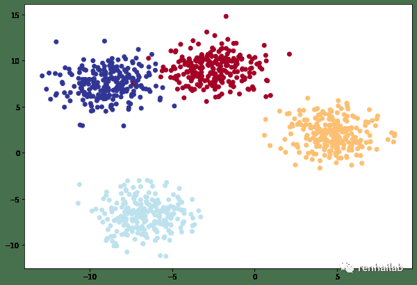
多类数据集
# Import dependencies
import torch
import matplotlib.pyplot as plt
from sklearn.datasets import make_blobs
from sklearn.model_selection import train_test_split

# 设置参数
NUM_CLASSES = 4 # 输出类
NUM_FEATURES = 2 # 输入特征
RANDOM_SEED = 42 # 随机种子

# 1. 创建多类分类数据
X_blob, y_blob = make_blobs(n_samples=1000,
    n_features=NUM_FEATURES, # X features
    centers=NUM_CLASSES, # y labels
    cluster_std=1.5, # 给与每个类的标准差
    random_state=RANDOM_SEED
)

# 2. 将数据转为tensor
X_blob = torch.from_numpy(X_blob).type(torch.float)
y_blob = torch.from_numpy(y_blob).type(torch.LongTensor)
print(X_blob[:5], y_blob[:5])

# 3. 分割数据
X_blob_train, X_blob_test, y_blob_train, y_blob_test = train_test_split(X_blob,
    y_blob,
    test_size=0.2,
    random_state=RANDOM_SEED
)

# 4. 绘制数据
plt.figure(figsize=(10, 7))
plt.scatter(X_blob[:, 0], X_blob[:, 1], c=y_blob, cmap=plt.cm.RdYlBu);
7.2 创建模型
# 5. 设置device
device = "cuda" if torch.cuda.is_available() else "cpu"

from torch import nn


# 6. 创建模型
class BlobModel(nn.Module):
    def __init__(self, input_features, output_features, hidden_units=8):
        """Initializes all required hyperparameters for a multi-class classification model.

        Args:
            input_features (int): Number of input features to the model.
            out_features (int): Number of output features of the model
              (how many classes there are).
            hidden_units (int): Number of hidden units between layers, default 8.
        """
        super().__init__()
        self.linear_layer_stack = nn.Sequential(
            nn.Linear(in_features=input_features, out_features=hidden_units),
            # nn.ReLU(), # <- does our dataset require non-linear layers? (try uncommenting and see if the results change)
            nn.Linear(in_features=hidden_units, out_features=hidden_units),
            # nn.ReLU(), # <- does our dataset require non-linear layers? (try uncommenting and see if the results change)
            nn.Linear(in_features=hidden_units, out_features=output_features),  # how many classes are there?
        )

    def forward(self, x):
        return self.linear_layer_stack(x)


# 7. 实例化模型
model_4 = BlobModel(input_features=NUM_FEATURES,
                    output_features=NUM_CLASSES,
                    hidden_units=8).to(device)
7.3 创建损失函数和优化器
# 创建一个损失函数
loss_fn = nn.CrossEntropyLoss()

# 创建一个优化器
optimizer = torch.optim.SGD(params=model_4.parameters(),
                            lr=0.1)
7.4 正式训练
torch.manual_seed(42)

# 设置迭代次数
epochs = 100

# 将数据传输到device(前文定义过)
X_blob_train, y_blob_train = X_blob_train.to(device), y_blob_train.to(device)
X_blob_test, y_blob_test = X_blob_test.to(device), y_blob_test.to(device)

# 计算准确度
def accuracy_fn(y_true, y_pred):
    correct = torch.eq(y_true, y_pred).sum().item()
    acc = (correct / len(y_pred)) * 100
    return acc

# 进行训练和评估循环
for epoch in range(epochs):
    ### 训练
    model_4.train()

    # 1. 向前传播
    y_logits = model_4(X_blob_train) #  model outputs raw logits
    y_pred = torch.softmax(y_logits, dim=1).argmax(dim=1) # 后文会说明

    # 2. 计算损失和准确度
    loss = loss_fn(y_logits, # 使用前文定义的nn.BCEWithLogitsLoss二元交叉熵损失
                   y_blob_train)
    acc = accuracy_fn(y_true=y_blob_train,
                      y_pred=y_pred)

    # 3. 归零梯度
    optimizer.zero_grad()

    # 4.通过进行反向传播来计算梯度
    loss.backward()

    # 5. 过调用优化器来更新模型参数
    optimizer.step()

    ### 测试
    model_4.eval()
    with torch.inference_mode():
        # 1. 向前传播
        test_logits = model_4(X_blob_test).squeeze()
        test_pred = torch.softmax(test_logits, dim=1).argmax(dim=1)

        # 2. 计算损失
        test_loss = loss_fn(test_logits,
                            y_blob_test)
        test_acc = accuracy_fn(y_true=y_blob_test,
                               y_pred=test_pred)

    # 10个循环输出一次结果
    if epoch % 10 == 0:
        print(f"Epoch: {epoch} | Loss: {loss:.5f}, Accuracy: {acc:.2f}% | Test loss: {test_loss:.5f}, Test acc: {test_acc:.2f}%")
首先解释:logits -> prediction probabilities -> prediction labels过程。
model_4(X_blob_train)执行了对输入数据X_blob_train的推理操作,返回了原始的 logits。Logits 是模型在每个类别上的得分或置信度,通常是未经归一化的结果。torch.softmax(y_logits, dim=1)将 logits 应用 softmax 函数,将其转换为概率分布。Softmax 函数可以将原始的实数值转换为范围在 0 到 1 之间的概率值,且所有类别的概率之和为 1。.argmax(dim=1)找到每个样本预测概率最高的类别索引,即预测标签。dim=1参数表示在每个样本的维度上执行argmax操作。
因此,y_pred 是通过将原始 logits 转换为概率分布,然后找到概率最高的类别索引而得到的预测标签。它是一个包含了每个样本的预测标签的张量。
7.5 进行预测和评估
我们开始预测:
# Make predictions
model_4.eval()
with torch.inference_mode():
    y_logits = model_4(X_blob_test)

# View the first 10 predictions
y_logits[:10]
tensor([[  4.3377,  10.3539, -14.8948,  -9.7642],
        [  5.0142, -12.0371,   3.3860,  10.6699],
        [ -5.5885, -13.3448,  20.9894,  12.7711],
        [  1.8400,   7.5599,  -8.6016,  -6.9942],
        [  8.0726,   3.2906, -14.5998,  -3.6186],
        [  5.5844, -14.9521,   5.0168,  13.2890],
        [ -5.9739, -10.1913,  18.8655,   9.9179],
        [  7.0755,  -0.7601,  -9.5531,   0.1736],
        [ -5.5918, -18.5990,  25.5309,  17.5799],
        [  7.3142,   0.7197, -11.2017,  -1.2011]], device='cuda:0')
将logits转为标签并 plot_decision_boundary()绘制出来:
# Turn predicted logits in prediction probabilities
y_pred_probs = torch.softmax(y_logits, dim=1)

# Turn prediction probabilities into prediction labels
y_preds = y_pred_probs.argmax(dim=1)

# Compare first 10 model preds and test labels
print(f"Predictions: {y_preds[:10]}\nLabels: {y_blob_test[:10]}")
print(f"Test accuracy: {accuracy_fn(y_true=y_blob_test, y_pred=y_preds)}%")
Predictions: tensor([1, 3, 2, 1, 0, 3, 2, 0, 2, 0], device='cuda:0')
Labels: tensor([1, 3, 2, 1, 0, 3, 2, 0, 2, 0], device='cuda:0')
Test accuracy: 99.5%
plt.figure(figsize=(12, 6))
plt.subplot(1, 2, 1)
plt.title("Train")
plot_decision_boundary(model_4, X_blob_train, y_blob_train)
plt.subplot(1, 2, 2)
plt.title("Test")
plot_decision_boundary(model_4, X_blob_test, y_blob_test)
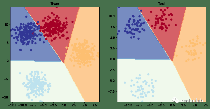
model_4 训练和结果
8.更多分类评估指标
指标名称 | 定义 | 代码 |
|---|---|---|
Accuracy 准确性 | 在 100 个预测中,您的模型有多少是正确的?例如,95% 的准确度意味着 95/100 的预测正确。 | `torchmetrics.Accuracy()`[38] or `sklearn.metrics.accuracy_score()`[39] |
Precision 精确度 | 真阳性(true positives)占样本总数的比例。精度越高,误报就越少(模型在本应为 0 的情况下却预测为 1)。 | `torchmetrics.Precision()`[40] `sklearn.metrics.precision_score()`[41] |
Recall | 真阳性占真阳性和假阴性总数的比例(模型预测本应为 1 的结果为 0)。更高的Recall 会导致更少的假阴性。 | `torchmetrics.Recall()`[42] or `sklearn.metrics.recall_score()`[43] |
F1-score | 将精确度和召回率合并为一个指标。1 是最好的,0 是最差的。 | `torchmetrics.F1Score()`[44] or `sklearn.metrics.f1_score()`[45] |
Confusion matrix 混淆矩阵[46] | 以表格方式比较预测值与真实值,如果 100% 正确,则矩阵中的所有值将从左上到右下(对角线)。 | `torchmetrics.ConfusionMatrix`[47] or `sklearn.metrics.plot_confusion_matrix()`[48] |
Classification report 分类报告 | 一些主要分类指标的集合,例如精度、召回率和 F1 分数。 | `sklearn.metrics.classification_report()`[49] |
注意:这是一个将英文翻译为中文的表格,其中包含了指标名称、定义和代码。
Scikit-Learn(一个流行的世界级机器学习库)有许多上述指标的实现, PyTorch 的版本的实现方式可以查看 TorchMetrics[50],尤其是 TorchMetrics 分类部分[51]。
让我们尝试一下 torchmetrics.Accuracy 方法。
try:
    from torchmetrics import Accuracy
except:
    !pip install torchmetrics==0.9.3 # this is the version we're using in this notebook (later versions exist here: https://torchmetrics.readthedocs.io/en/stable/generated/CHANGELOG.html#changelog)
    from torchmetrics import Accuracy

# 确保数据在同一个device
torchmetrics_accuracy = Accuracy(task='multiclass', num_classes=4).to(device)

# 计算 accuracy
torchmetrics_accuracy(y_preds, y_blob_test)

>>>
tensor(0.9950, device='cuda:0')
感谢
感谢原作者 Daniel Bourke,访问https://www.learnpytorch.io/[52]可以阅读英文原文,点击原作者的Github仓库:https://github.com/mrdbourke/pytorch-deep-learning/[53]可以获得帮助和其他信息。
本文同样遵守遵守 MIT license[54],不受任何限制,包括但不限于权利
使用、复制、修改、合并、发布、分发、再许可和/或出售。但需标明原始作者的许可信息:renhai-lab:https://cdn.renhai-lab.tech/。
参考资料
[1]
PyTorch Neural Network Classification: https://www.learnpytorch.io/02_pytorch_classification/
[2]
《使用PyTorch进行深度学习系列》课程介绍: https://cdn.renhai-lab.tech/archives/DL-Home
[3]
我的博客: https://cdn.renhai-lab.tech/categories/deep-learning
[4]
阅读原文: https://cdn.renhai-lab.tech/archives/DL-03-pytorch_classification
[5]
深度学习之神经网络的结构的视频(强烈建议观看): https://www.bilibili.com/video/BV1bx411M7Zx/?share_source=copy_web&vd_source=bbeafbcfe326916409d46b815d8cb3a3
[6]
ReLU: https://pytorch.org/docs/stable/generated/torch.nn.ReLU.html#torch.nn.ReLU
[7]
torch.sigmoid: https://pytorch.org/docs/stable/generated/torch.sigmoid.html
[8]
torch.softmax: https://pytorch.org/docs/stable/generated/torch.nn.Softmax.html
[9]
torch.nn.CrossEntropyLoss: https://pytorch.org/docs/stable/generated/torch.nn.CrossEntropyLoss.html
[10]
SGD: https://pytorch.org/docs/stable/generated/torch.optim.SGD.html
[11]
Adam: https://pytorch.org/docs/stable/generated/torch.optim.Adam.html
[12]
torch.optim: https://pytorch.org/docs/stable/optim.html
[13]
make_circles(): https://scikit-learn.org/stable/modules/generated/sklearn.datasets.make_circles.html
[14]
train_test_split(): https://scikit-learn.org/stable/modules/generated/sklearn.model_selection.train_test_split.html
[15]
TensorFlow Playground: https://playground.tensorflow.org/
[16]
torch.optim.SGD(): https://pytorch.org/docs/stable/generated/torch.optim.SGD.html
[17]
torch.optim.Adam(): https://pytorch.org/docs/stable/generated/torch.optim.Adam.html
[18]
torch.nn.BCELossWithLogits: https://pytorch.org/docs/stable/generated/torch.nn.BCEWithLogitsLoss.html
[19]
torch.nn.BCELoss: https://pytorch.org/docs/stable/generated/torch.nn.BCELoss.html
[20]
torch.nn.CrossEntropyLoss: https://pytorch.org/docs/stable/generated/torch.nn.CrossEntropyLoss.html
[21]
torch.nn.L1Loss: https://pytorch.org/docs/stable/generated/torch.nn.L1Loss.html
[22]
torch.nn.MSELoss: https://pytorch.org/docs/stable/generated/torch.nn.MSELoss.html#torch.nn.MSELoss
[23]
torch.nn.BCELoss(): https://pytorch.org/docs/stable/generated/torch.nn.BCELoss.html
[24]
torch.nn.BCEWithLogitsLoss(): https://pytorch.org/docs/stable/generated/torch.nn.BCEWithLogitsLoss.html
[25]
torch.nn.BCEWithLogitsLoss() 的文档: https://pytorch.org/docs/stable/generated/torch.nn.BCEWithLogitsLoss.html
[26]
PyTorch工作流程基础知识【PyTorch 深度学习系列】: https://cdn.renhai-lab.tech/archives/DL-02-pytorch-workflow
[27]
sigmoid 激活函数: https://pytorch.org/docs/stable/special.html#torch.special.expit
[28]
softmax 激活函数: https://pytorch.org/docs/stable/generated/torch.nn.Softmax.html
[29]
Learn PyTorch for Deep Learning 存储库: https://github.com/mrdbourke/pytorch-deep-learning
[30]
helper_functions.py: https://github.com/mrdbourke/pytorch-deep-learning/blob/main/helper_functions.py
[31]
06-PyTorch迁移学习:在预训练模型上进行训练: https://cdn.renhai-lab.tech/archives/DL-06-pytorch-transfer_learning
[32]
原文: https://www.learnpytorch.io/02_pytorch_classification/#5-improving-a-model-from-a-model-perspective
[33]
现成的非线性激活函数: https://pytorch.org/docs/stable/nn.html#non-linear-activations-weighted-sum-nonlinearity
[34]
torch.nn.ReLU(): https://pytorch.org/docs/stable/generated/torch.nn.ReLU.html
[35]
ImageNet-1k: https://www.image-net.org/
[36]
sklearn.datasets: https://scikit-learn.org/stable/modules/classes.html#module-sklearn.datasets
[37]
make_blobs(): https://scikit-learn.org/stable/modules/generated/sklearn.datasets.make_blobs.html
[38]
torchmetrics.Accuracy(): https://torchmetrics.readthedocs.io/en/stable/classification/accuracy.html#id3
[39]
sklearn.metrics.accuracy_score(): https://scikit-learn.org/stable/modules/generated/sklearn.metrics.accuracy_score.html
[40]
torchmetrics.Precision(): https://torchmetrics.readthedocs.io/en/stable/classification/precision.html#id4
[41]
sklearn.metrics.precision_score(): https://scikit-learn.org/stable/modules/generated/sklearn.metrics.precision_score.html
[42]
torchmetrics.Recall(): https://torchmetrics.readthedocs.io/en/stable/classification/recall.html#id5
[43]
sklearn.metrics.recall_score(): https://scikit-learn.org/stable/modules/generated/sklearn.metrics.recall_score.html
[44]
torchmetrics.F1Score(): https://torchmetrics.readthedocs.io/en/stable/classification/f1_score.html#f1score
[45]
sklearn.metrics.f1_score(): https://scikit-learn.org/stable/modules/generated/sklearn.metrics.f1_score.html
[46]
Confusion matrix 混淆矩阵: https://www.dataschool.io/simple-guide-to-confusion-matrix-terminology/
[47]
torchmetrics.ConfusionMatrix: https://torchmetrics.readthedocs.io/en/stable/classification/confusion_matrix.html#confusionmatrix
[48]
sklearn.metrics.plot_confusion_matrix(): https://scikit-learn.org/stable/modules/generated/sklearn.metrics.ConfusionMatrixDisplay.html#sklearn.metrics.ConfusionMatrixDisplay.from_predictions
[49]
sklearn.metrics.classification_report(): https://scikit-learn.org/stable/modules/generated/sklearn.metrics.classification_report.html
[50]
TorchMetrics: https://torchmetrics.readthedocs.io/en/latest/
[51]
TorchMetrics 分类部分: https://torchmetrics.readthedocs.io/en/stable/pages/classification.html
[52]
https://www.learnpytorch.io/: https://www.learnpytorch.io/
[53]
https://github.com/mrdbourke/pytorch-deep-learning/: https://github.com/mrdbourke/pytorch-deep-learning/
[54]
MIT license: https://github.com/renhai-lab/pytorch-deep-learning/blob/cb770bbe688f5950421a76c8b3a47aaa00809c8c/LICENSE
[55]
我的博客: https://cdn.renhai-lab.tech/
[56]
我的GITHUB: https://github.com/renhai-lab
[57]
我的GITEE: https://gitee.com/renhai-lab
[58]
我的知乎: https://www.zhihu.com/people/Ing_ideas
腾讯云开发者
