多层感知机(MLP):从数学原理到实战应用


在这里插入图片描述
前言
在人工智能和机器学习的广阔领域中,多层感知机(Multilayer Perceptron, MLP)作为神经网络家族中最基础且最具代表性的成员,承载着特殊的历史地位和技术价值。从1958年Rosenblatt提出感知机概念,到如今MLP成为现代深度学习架构的核心组件,这一简洁而强大的模型始终在人工智能发展历程中扮演着关键角色。
本文旨在提供一个全面而深入的MLP学习指南,从严谨的数学定义出发,通过清晰的代码实现,到实际的应用案例,系统性地展现MLP的理论基础、实现技巧和应用前景。无论您是机器学习初学者,还是寻求深入理解神经网络数学原理的研究者,或是希望将MLP应用到实际问题的工程师,本文都将为您提供有价值的参考。
在阅读本文的过程中,您将逐步掌握MLP的数学表述、前向与反向传播算法、各类优化技巧,以及在分类、回归等任务中的实战应用。更重要的是,您将理解为什么在深度学习蓬勃发展的今天,MLP仍然是连接传统机器学习与现代深度学习的重要桥梁,以及它如何与最新的深度学习架构融合,继续发挥其不可替代的作用。
让我们一起探索这个看似简单却蕴含深刻智慧的神经网络模型,揭开它的数学之美与实用之道。
导读目录
- 基本定义
- MLP的概念与结构
- 历史发展沿革
- 数学表述
- 网络结构的数学描述
- 参数定义(权重矩阵与偏置向量)
- 前向传播算法
- 激活函数比较
- 损失函数选择
- 反向传播算法
- 激活函数与损失函数的区别
- 向量化表示
- 批量数据处理
- 矩阵运算优化
- 函数逼近能力
- 通用逼近定理
- MLP的表达能力
- MLP实现分类任务实战
- 鸢尾花数据集分类
- MLP模型实现
- 网络训练与评估
- MLP实现回归任务实战
- 波士顿房价预测
- 回归MLP模型
- 训练与评估指标
- MLP在工业界的高级应用
- 信用卡欺诈检测
- 推荐系统中的特征嵌入
- MLP优化高级技巧
- 权重初始化策略
- 正则化技术组合
- 学习率调度策略
- MLP与深度学习新架构的融合
- Transformer中的MLP模块
- 图神经网络中的特征变换
- MLP的局限与未来
- 本质局限性
- 未来发展方向
- 结语:永恒的神经网络基石
在深度学习的世界里,有一种基础却强大的模型始终闪耀着独特光芒——它就是多层感知机(MLP)。
作为前馈神经网络的核心代表,MLP以其优雅的结构和强大的表达能力,成为解决分类与回归问题的通用框架。本文将带您从数学原理到代码实现,全面探索这一深度学习基石模型的奥秘。
1. 基本定义
多层感知机(Multilayer Perceptron, MLP)是一种前馈人工神经网络,由多层节点组成,每层节点与下一层的节点全连接。除了输入层外,每个节点都是一个使用非线性激活函数的神经元。MLP至少包含三层:输入层、一个或多个隐藏层和输出层。 其历史发展沿革为从单层到多层,实现历史性跨越: 1958年:Frank Rosenblatt提出感知机,只能解决线性可分问题
1969年:Minsky证明单层网络无法解决异或问题,AI进入寒冬
1986年:Rumelhart提出反向传播算法,MLP重获新生
2023年:MLP在Transformer等现代架构中扮演关键角色
2. 数学表述
2.1 网络结构
假设一个具有
层的MLP,其中:
- 第0层是输入层,有
个节点
- 第1到
层是隐藏层,第
层有
个节点
- 第
层是输出层,有
个节点
2.2 参数定义
对于每一层
,MLP定义了以下参数:
- 权重矩阵
:
表示从第
层的第
个节点到第
层的第
个节点的连接权重
- 偏置向量
:
表示第
层的第
个节点的偏置
2.3 前向传播
给定输入向量
,MLP的前向传播过程如下:
- 初始化:
(输入层的激活值就是输入向量)
- 对于每一层
,计算:
- 线性变换:
- 激活函数:
其中
是第
层的激活函数,常用的激活函数包括:
- Sigmoid函数:
- Tanh函数:
- ReLU函数:
- Leaky ReLU函数:
,其中
是一个小正数
- 输出:
(网络的预测输出)
用矩阵表示,对于一批样本
(
是样本数量),前向传播可以表示为:
- 对于
:
激活函数的选择可以参考如下:
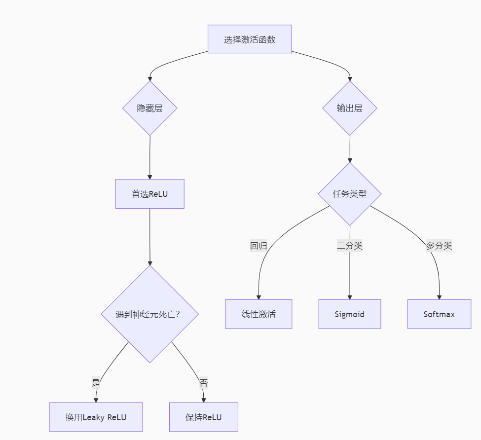
在这里插入图片描述
常用激活函数对比
函数 | 公式 | 导数 | 优点 | 缺点 |
|---|---|---|---|---|
Sigmoid | 11+e−x\frac{1}{1+e^{-x}}1+e−x1 | σ(x)(1−σ(x))\sigma(x)(1-\sigma(x))σ(x)(1−σ(x)) | 输出平滑 | 梯度消失 |
Tanh | ex−e−xex+e−x\frac{e^x - e^{-x}}{e^x + e^{-x}}ex+e−xex−e−x | 1−tanh2(x)1 - \tanh^2(x)1−tanh2(x) | 零中心化 | 梯度消失 |
ReLU | max(0,x)\max(0,x)max(0,x) | 1 if x>0 else 01 \text{ if } x>0 \text{ else } 01 if x>0 else 0 | 计算高效 | 神经元死亡 |
Leaky ReLU | max(0.01x,x)\max(0.01x, x)max(0.01x,x) | 1 if x>0 else 0.011 \text{ if } x>0 \text{ else } 0.011 if x>0 else 0.01 | 解决死亡问题 | 非零斜率 |
输出平滑梯度消失Tanh
零中心化梯度消失ReLU
计算高效神经元死亡Leaky ReLU
解决死亡问题非零斜率
2.4 损失函数
为了训练MLP,需要定义一个损失函数来衡量预测输出与真实标签之间的差距。常用的损失函数包括:
- 均方误差(MSE):用于回归问题
- 交叉熵损失:用于分类问题
其中
是第
个样本的真实标签,
是对应的预测输出。
我们正在讨论神经网络的两个核心概念:激活函数和损失函数。它们虽然都是函数,但在神经网络中扮演着完全不同的角色。下面我将详细解释它们的区别,包括定义、作用、位置以及示例。下面我们做一个小的展开:
- 激活函数(Activation Function):
- 定义:激活函数是作用于神经网络中神经元输出的函数,它将神经元的输入(加权和加上偏置)映射到输出。
- 作用:
- 引入非线性:使神经网络能够学习和表示复杂的数据模式(如果没有非线性激活函数,多层网络将退化为单层线性模型)。
- 决定神经元是否被激活:通过将输出压缩到特定范围(如Sigmoid函数将输出压缩到0-1之间)或过滤掉某些值(如ReLU函数将负值置零)。
- 位置:通常位于神经网络的隐藏层和输出层(但输出层的激活函数有时会根据任务选择不同的形式)。
- 常见类型:
- Sigmoid: 将输入压缩到(0,1)区间,常用于二分类的输出层。
- Tanh: 将输入压缩到(-1,1)区间,具有零中心化特性。
- ReLU: 对于正值输出原值,负值输出0,计算高效,缓解梯度消失(但可能导致神经元死亡)。
- Softmax: 将多个神经元的输出转化为概率分布,常用于多分类的输出层。
- 损失函数(Loss Function):
- 定义:损失函数(也称为代价函数)用于衡量模型预测值与真实值之间的差异。它是模型训练过程中需要最小化的目标函数。
- 作用:
- 量化误差:为模型提供反馈,指示预测结果与真实结果的偏差程度。
- 指导优化:通过梯度下降等优化算法,损失函数的梯度被用来更新网络权重,从而逐步减小误差。
- 位置:损失函数位于整个神经网络的输出端,用于计算预测结果与真实标签之间的差异。
- 常见类型:
- 均方误差(MSE):用于回归问题,计算预测值与真实值之差的平方的平均值。
- 交叉熵损失(Cross-Entropy):用于分类问题,特别是二分类(Binary Cross-Entropy)和多分类(Categorical Cross-Entropy)。
- 铰链损失(Hinge Loss):常用于支持向量机(SVM)和某些分类任务。
- 主要区别总结: 特点激活函数损失函数目的引入非线性,决定神经元输出衡量模型预测与真实值的差距作用位置神经元的输出端(隐藏层和输出层)整个网络的输出端(计算预测和标签的差异)输入神经元的加权输入(线性组合)模型的最终预测输出和真实标签输出神经元的激活输出(作为下一层的输入)一个标量值(表示误差大小)示例ReLU, Sigmoid, Tanh, SoftmaxMSE, Cross-Entropy, Hinge Loss
- 示例说明:
考虑一个简单的二分类神经网络:
- 输入层:2个神经元
- 隐藏层:3个神经元(使用ReLU激活函数)
- 输出层:1个神经元(使用Sigmoid激活函数)
- 损失函数:二元交叉熵(Binary Cross-Entropy) 前向传播过程: 隐藏层输入:h_in = X * W1 + b1 隐藏层输出:h_out = ReLU(h_in) 输出层输入:o_in = h_out * W2 + b2 输出层输出:o_out = Sigmoid(o_in) # 预测概率 然后计算损失: 损失值 = BinaryCrossEntropy(y_true, o_out) 反向传播时: 先计算损失函数对输出层输出的梯度,然后反向传播到输出层的输入(即Sigmoid的输入),再继续反向传播到隐藏层的输出,然后到隐藏层的输入(即ReLU的输入),最后到权重和偏置。
- 为什么需要两者?
- 激活函数:使网络具备非线性建模能力,没有它,无论多少层都只能表示线性关系。
- 损失函数:提供优化目标,没有它,网络无法知道预测结果的好坏,也无法调整参数。 通过以上解释,我们可以清楚地看到激活函数和损失函数在神经网络中的不同角色和重要性。激活函数是神经元内部的转换函数,而损失函数是整个网络性能的评估标准。
2.5 反向传播
反向传播算法用于计算损失函数对各参数的梯度,以便使用梯度下降法更新参数。对于一个样本,反向传播的过程如下:
- 输出层误差:
其中
是损失函数对输出层激活值的梯度,
是输出层激活函数的导数,
表示元素wise乘法。
- 隐藏层误差(从后向前传播): 对于
:
- 计算梯度: 对于
:
- 参数更新(梯度下降):
其中
是学习率。
对于一批样本,梯度是所有样本梯度的平均值。
3. 向量化表示
为了提高计算效率,通常使用向量化实现MLP。对于一批包含
个样本的数据:
- 输入:
,其中每列是一个样本
- 真实标签:
- 前向传播:
A[0]=XA^{[0]} = X - 对于
l∈{1,2,...,L}l \in \{1, 2, ..., L\} :
Z[l]=W[l]A[l−1]+b[l]Z^{[l]} = W^{[l]} A^{[l-1]} + b^{[l]} A[l]=g[l](Z[l])A^{[l]} = g^{[l]}(Z^{[l]}) Y^=A[L]\hat{Y} = A^{[L]} - 损失函数:
- MSE:
JMSE=1m∑i=1m∥Y(i)−Y^(i)∥2J_{MSE} = \frac{1}{m} \sum_{i=1}^{m} \|Y^{(i)} - \hat{Y}^{(i)}\|^2 - 交叉熵:
JCE=−1m∑i=1m∑j=1n[L]Yjilog(Y^ji)J_{CE} = -\frac{1}{m} \sum_{i=1}^{m} \sum_{j=1}^{n^{[L]}} Y_{ji} \log(\hat{Y}_{ji}) - 反向传播:
δ[L]=1m(Y^−Y)⊙g′[L](Z[L])\delta^{[L]} = \frac{1}{m}(\hat{Y} - Y) \odot g'^{[L]}(Z^{[L]}) - 对于
l∈{L−1,L−2,...,1}l \in \{L-1, L-2, ..., 1\} :
δ[l]=(W[l+1])Tδ[l+1]⊙g′[l](Z[l])\delta^{[l]} = (W^{[l+1]})^T \delta^{[l+1]} \odot g'^{[l]}(Z^{[l]}) - 对于
l∈{1,2,...,L}l \in \{1, 2, ..., L\} :
∇W[l]J=δ[l](A[l−1])T\nabla_{W^{[l]}} J = \delta^{[l]} (A^{[l-1]})^T ∇b[l]J=∑i=1mδi[l]\nabla_{b^{[l]}} J = \sum_{i=1}^{m} \delta^{[l]}_i
4. 函数逼近能力
MLP的一个重要理论基础是通用逼近定理(Universal Approximation Theorem),该定理表明:
具有单一隐藏层和有限数量神经元的前馈神经网络,可以以任意精度逼近任何连续函数,只要给予足够数量的隐藏单元和适当的权重。
这意味着理论上,MLP可以学习任何连续函数映射,这使得它在各种机器学习任务中都具有广泛的应用。
多层感知机可以表示为一个函数
,该函数由一系列线性变换和非线性激活函数组成:
这个函数通过最小化损失函数
来学习最优参数
和
。
5. MLP实现分类任务实战
在理解了MLP的数学基础后,我们可以通过实际案例来展示如何使用MLP解决分类问题。本节将使用经典的鸢尾花数据集来实现一个多类分类任务。
5.1 鸢尾花分类数据集
鸢尾花数据集是机器学习中最著名的数据集之一,包含三种不同品种的鸢尾花的测量特征。每个样本有四个特征:萼片长度、萼片宽度、花瓣长度和花瓣宽度。我们的目标是根据这些特征将鸢尾花分类为三个不同的品种。
首先,我们需要加载和预处理数据:
import numpy as np
from sklearn.datasets import load_iris
from sklearn.preprocessing import StandardScaler
from sklearn.model_selection import train_test_split

# 加载数据
iris = load_iris()
X = iris.data
y = iris.target

# 数据标准化 - 对模型训练非常重要
scaler = StandardScaler()
X = scaler.fit_transform(X)

# 将标签转换为独热编码形式
y_onehot = np.eye(3)[y]

# 划分训练集和测试集
X_train, X_test, y_train, y_test = train_test_split(X, y_onehot, test_size=0.2, random_state=42)
数据预处理是机器学习中的关键步骤。标准化可以使不同尺度的特征具有相同的影响力,独热编码则将类别标签转换为适合神经网络处理的形式。
5.2 MLP模型实现
接下来,我们实现一个简单的MLP类,包含一个隐藏层:
class MLP:
    def __init__(self, input_size, hidden_size, output_size):
        # 初始化权重和偏置
        self.W1 = np.random.randn(input_size, hidden_size) * 0.01
        self.b1 = np.zeros((1, hidden_size))
        self.W2 = np.random.randn(hidden_size, output_size) * 0.01
        self.b2 = np.zeros((1, output_size))

    def relu(self, x):
        return np.maximum(0, x)

    def relu_derivative(self, x):
        return np.where(x > 0, 1, 0)

    def softmax(self, x):
        exp_x = np.exp(x - np.max(x, axis=1, keepdims=True))  # 防止数值溢出
        return exp_x / np.sum(exp_x, axis=1, keepdims=True)

    def forward(self, X):
        # 前向传播
        self.z1 = np.dot(X, self.W1) + self.b1
        self.a1 = self.relu(self.z1)
        self.z2 = np.dot(self.a1, self.W2) + self.b2
        self.a2 = self.softmax(self.z2)
        return self.a2

    def backward(self, X, y, learning_rate):
        # 反向传播
        m = X.shape[0]

        # 输出层误差
        dz2 = self.a2 - y
        dW2 = (1/m) * np.dot(self.a1.T, dz2)
        db2 = (1/m) * np.sum(dz2, axis=0, keepdims=True)

        # 隐藏层误差
        dz1 = np.dot(dz2, self.W2.T) * self.relu_derivative(self.z1)
        dW1 = (1/m) * np.dot(X.T, dz1)
        db1 = (1/m) * np.sum(dz1, axis=0, keepdims=True)

        # 更新参数
        self.W2 -= learning_rate * dW2
        self.b2 -= learning_rate * db2
        self.W1 -= learning_rate * dW1
        self.b1 -= learning_rate * db1
5.3 网络训练与评估
现在我们可以训练我们的MLP模型并评估其性能:
# 定义交叉熵损失函数
def cross_entropy_loss(y_pred, y_true):
    m = y_true.shape[0]
    epsilon = 1e-8  # 防止对数中的零值
    y_pred = np.clip(y_pred, epsilon, 1 - epsilon)
    log_likelihood = -np.sum(y_true * np.log(y_pred)) / m
    return log_likelihood

# 创建MLP
mlp = MLP(input_size=4, hidden_size=10, output_size=3)

# 训练参数
epochs = 5000
lr = 0.01

# 训练循环
for epoch in range(epochs):
    # 前向传播
    output = mlp.forward(X_train)

    # 计算损失 (交叉熵)
    loss = cross_entropy_loss(output, y_train)

    # 反向传播
    mlp.backward(X_train, y_train, lr)

    # 每500轮打印损失
    if epoch % 500 == 0:
        print(f"Epoch {epoch}, Loss: {loss:.4f}")

# 评估
test_output = mlp.forward(X_test)
predictions = np.argmax(test_output, axis=1)
true_labels = np.argmax(y_test, axis=1)
accuracy = np.mean(predictions == true_labels)
print(f"Test Accuracy: {accuracy*100:.2f}%")
在这个训练过程中,我们使用了交叉熵损失函数,这是分类问题的标准选择。随着训练的进行,损失值应该会逐渐减小,而准确率会提高。一个训练良好的模型在这个简单的数据集上通常可以达到95%以上的准确率。
6. MLP实现回归任务实战
除了分类问题,MLP也非常适合解决回归问题。在本节中,我们将使用MLP来预测波士顿房价数据集中的房价。
6.1 波士顿房价预测
波士顿房价数据集包含了波士顿不同地区的房屋信息和对应的价格。每个样本有13个特征,如犯罪率、房间数量、高速公路可达性等。我们的目标是预测房屋价格。
import numpy as np
from sklearn.datasets import fetch_california_housing  # 注:load_boston已被弃用,使用california_housing替代
from sklearn.preprocessing import StandardScaler
from sklearn.model_selection import train_test_split

# 加载数据
housing = fetch_california_housing()
X = housing.data
y = housing.target.reshape(-1, 1)

# 标准化特征和目标值
X_scaler = StandardScaler()
y_scaler = StandardScaler()
X = X_scaler.fit_transform(X)
y = y_scaler.fit_transform(y)

# 划分数据集
X_train, X_test, y_train, y_test = train_test_split(X, y, test_size=0.2, random_state=42)
y_test_original = y_scaler.inverse_transform(y_test)  # 保存原始比例的测试集标签,用于后续评估
对于回归问题,我们需要对目标变量也进行标准化,这有助于模型更快地收敛。
6.2 回归MLP模型
回归MLP与分类MLP的主要区别在于输出层不使用激活函数(或使用线性激活函数),并且使用均方误差(MSE)作为损失函数:
class RegressionMLP(MLP):
    def __init__(self, input_size, hidden_size, output_size):
        super().__init__(input_size, hidden_size, output_size)

    def forward(self, X):
        # 前向传播
        self.z1 = np.dot(X, self.W1) + self.b1
        self.a1 = self.relu(self.z1)
        self.z2 = np.dot(self.a1, self.W2) + self.b2
        return self.z2  # 线性输出,不使用激活函数

    def backward(self, X, y, learning_rate):
        # 反向传播
        m = X.shape[0]

        # 输出层误差 (使用MSE损失)
        dz2 = (self.z2 - y) / m
        dW2 = np.dot(self.a1.T, dz2)
        db2 = np.sum(dz2, axis=0, keepdims=True)

        # 隐藏层误差
        dz1 = np.dot(dz2, self.W2.T) * self.relu_derivative(self.z1)
        dW1 = np.dot(X.T, dz1)
        db1 = np.sum(dz1, axis=0, keepdims=True)

        # 更新参数
        self.W2 -= learning_rate * dW2
        self.b2 -= learning_rate * db2
        self.W1 -= learning_rate * dW1
        self.b1 -= learning_rate * db1
6.3 训练与评估指标
对于回归问题,我们通常使用均方误差(MSE)作为训练损失,使用R²分数来评估模型性能:
# 训练模型
mlp = RegressionMLP(input_size=X.shape[1], hidden_size=20, output_size=1)

# 训练参数
epochs = 10000
lr = 0.001

# 训练循环
for epoch in range(epochs):
    # 前向传播
    pred = mlp.forward(X_train)

    # 计算损失 (MSE)
    loss = np.mean((pred - y_train)**2)

    # 反向传播
    mlp.backward(X_train, y_train, lr)

    # 每1000轮打印损失
    if epoch % 1000 == 0:
        print(f"Epoch {epoch}, MSE Loss: {loss:.4f}")

# 预测测试集
test_pred = mlp.forward(X_test)

# 将预测结果转换回原始比例
test_pred = y_scaler.inverse_transform(test_pred)

# 评估模型性能
from sklearn.metrics import r2_score, mean_squared_error
r2 = r2_score(y_test_original, test_pred)
rmse = np.sqrt(mean_squared_error(y_test_original, test_pred))
print(f"R-squared: {r2:.4f}")
print(f"RMSE: {rmse:.4f}")
R²分数表示模型解释的方差比例,值越接近1表示模型性能越好。均方根误差(RMSE)提供了预测误差的直观度量,单位与目标变量相同。
在实际应用中,我们可能还需要考虑其他因素,如模型复杂度、训练时间和可解释性。对于更复杂的回归问题,可能需要更深的网络结构或更先进的优化技术。
7. MLP在工业界的高级应用
MLP在工业界有广泛的应用,从金融风控到推荐系统。本节将介绍两个实际应用案例,展示MLP如何解决复杂的现实问题。
7.1 信用卡欺诈检测
信用卡欺诈检测是一个典型的不平衡分类问题,因为欺诈交易通常只占所有交易的很小一部分。在这种情况下,我们需要特殊的技术来处理类别不平衡问题。
import tensorflow as tf
from tensorflow.keras.models import Sequential
from tensorflow.keras.layers import Dense, Dropout
from tensorflow.keras.optimizers import Adam
from tensorflow.keras.metrics import AUC

# 构建处理不平衡数据的MLP模型
def build_fraud_detection_model(input_dim=30):
    model = Sequential([
        Dense(64, input_dim=input_dim, activation='relu'),
        Dropout(0.5),  # 防止过拟合
        Dense(32, activation='relu'),
        Dropout(0.3),
        Dense(1, activation='sigmoid')  # 二分类问题
    ])

    # 焦点损失函数 - 专为处理不平衡数据设计
    def focal_loss(y_true, y_pred, alpha=0.25, gamma=2):
        """
        焦点损失:对难以分类的样本给予更高的权重
        - alpha: 平衡正负样本的权重
        - gamma: 调整难易样本的权重
        """
        pt = tf.where(tf.equal(y_true, 1), y_pred, 1 - y_pred)
        focal_weight = alpha * tf.pow(1 - pt, gamma)
        return -focal_weight * tf.math.log(pt)

    # 编译模型
    model.compile(
        optimizer=Adam(learning_rate=0.001),
        loss=focal_loss,
        metrics=[AUC()]  # AUC是不平衡数据的良好评估指标
    )

    return model

# 模型训练示例
# model = build_fraud_detection_model()
# history = model.fit(
#     X_train, y_train,
#     validation_data=(X_val, y_val),
#     class_weight={0: 1, 1: 50},  # 类别权重
#     batch_size=256,
#     epochs=20
# )
在欺诈检测中,我们使用了几种技术来处理不平衡数据:
- Dropout层:防止模型过拟合少数类
- 焦点损失:对难以分类的样本给予更高权重
- 类别权重:在训练时对少数类赋予更高权重
- AUC指标:比准确率更适合评估不平衡分类问题
7.2 推荐系统中的特征嵌入
推荐系统通常需要处理大量的类别特征(如用户ID、物品ID)。MLP可以与嵌入层结合,有效地学习这些特征的低维表示。
import tensorflow as tf
from tensorflow.keras.models import Model
from tensorflow.keras.layers import Input, Embedding, Flatten, Concatenate, Dense

def build_recommendation_model(num_users, num_items, embedding_size=16):
    # 输入层
    user_input = Input(shape=(1,), name='user_input')
    item_input = Input(shape=(1,), name='item_input')

    # 嵌入层 - 将用户和物品ID转换为密集向量
    user_embedding = Embedding(
        input_dim=num_users + 1,  # +1 用于处理未知用户
        output_dim=embedding_size,
        name='user_embedding'
    )(user_input)

    item_embedding = Embedding(
        input_dim=num_items + 1,  # +1 用于处理未知物品
        output_dim=embedding_size,
        name='item_embedding'
    )(item_input)

    # 展平嵌入向量
    user_vector = Flatten()(user_embedding)
    item_vector = Flatten()(item_embedding)

    # 合并特征
    merged = Concatenate()([user_vector, item_vector])

    # MLP层 - 学习用户-物品交互
    x = Dense(128, activation='relu')(merged)
    x = Dense(64, activation='relu')(x)
    x = Dense(32, activation='relu')(x)

    # 输出层 - 预测评分或点击概率
    output = Dense(1, activation='linear')(x)

    # 构建模型
    model = Model(inputs=[user_input, item_input], outputs=output)
    model.compile(optimizer='adam', loss='mean_squared_error')

    return model

# 模型使用示例
# model = build_recommendation_model(num_users=10000, num_items=5000)
# model.fit([user_ids, item_ids], ratings, epochs=10, batch_size=64)
这个推荐系统模型的关键特点是:
- 嵌入层:将高维稀疏的用户/物品ID转换为低维密集向量
- 特征融合:将用户和物品嵌入向量连接起来
- 多层MLP:学习用户和物品之间的复杂非线性交互
在实际应用中,这种模型通常会结合更多特征,如用户人口统计信息、物品属性、上下文信息等,以提高推荐的准确性和相关性。
8. MLP优化高级技巧
为了获得最佳性能,MLP模型通常需要各种优化技巧。本节将介绍几种提高MLP性能的高级技术。
8.1 权重初始化策略
权重初始化对模型的收敛速度和最终性能有重大影响。不同的激活函数适合不同的初始化方法:
方法 | 公式 | 适用场景 |
|---|---|---|
Xavier/Glorot | W∼U[−6nin+nout,6nin+nout]W \sim U[-\frac{\sqrt{6}}{\sqrt{n_{in}+n_{out}}}, \frac{\sqrt{6}}{\sqrt{n_{in}+n_{out}}}]W∼U[−nin+nout6,nin+nout6] | Tanh/Sigmoid |
He | W∼N(0,2nin)W \sim N(0, \sqrt{\frac{2}{n_{in}}})W∼N(0,nin2) | ReLU及其变体 |
LeCun | W∼N(0,1nin)W \sim N(0, \sqrt{\frac{1}{n_{in}}})W∼N(0,nin1) | SELU |
Tanh/SigmoidHe
ReLU及其变体LeCun
SELU
这些初始化方法的目标是保持每一层的方差相对恒定,防止梯度消失或爆炸。以下是实现示例:
import numpy as np
import tensorflow as tf
from tensorflow.keras.models import Sequential
from tensorflow.keras.layers import Dense
from tensorflow.keras.initializers import GlorotUniform, HeNormal, LecunNormal

# Xavier/Glorot初始化
model_xavier = Sequential([
    Dense(128, input_dim=20, activation='tanh',
          kernel_initializer=GlorotUniform()),
    Dense(64, activation='tanh',
          kernel_initializer=GlorotUniform()),
    Dense(1, activation='sigmoid')
])

# He初始化
model_he = Sequential([
    Dense(128, input_dim=20, activation='relu',
          kernel_initializer=HeNormal()),
    Dense(64, activation='relu',
          kernel_initializer=HeNormal()),
    Dense(1, activation='sigmoid')
])

# LeCun初始化
model_lecun = Sequential([
    Dense(128, input_dim=20, activation='selu',
          kernel_initializer=LecunNormal()),
    Dense(64, activation='selu',
          kernel_initializer=LecunNormal()),
    Dense(1, activation='sigmoid')
])
8.2 正则化技术组合
正则化技术可以防止过拟合,提高模型的泛化能力。多种正则化技术的组合通常比单独使用一种技术效果更好:
from tensorflow.keras.layers import BatchNormalization, Dropout
from tensorflow.keras.regularizers import l1, l2, l1_l2

def build_regularized_model(input_dim, output_dim):
    model = Sequential([
        # L2权重正则化 - 惩罚大的权重值
        Dense(128, input_dim=input_dim, activation='relu',
              kernel_regularizer=l2(0.01)),

        # Dropout - 随机关闭一定比例的神经元
        Dropout(0.3),

        # 批归一化 - 标准化每一层的输入
        BatchNormalization(),

        # 组合L1和L2正则化(弹性网络)
        Dense(64, activation='relu',
              kernel_regularizer=l1_l2(l1=0.001, l2=0.01)),

        Dropout(0.2),

        Dense(output_dim, activation='softmax')
    ])

    return model
每种正则化技术都有不同的作用:
- L1正则化:产生稀疏权重,有助于特征选择
- L2正则化:防止权重变得过大,平滑模型
- Dropout:通过训练过程中随机丢弃神经元来防止共适应
- 批归一化:标准化每一层的输入,加速训练并提高稳定性
8.3 学习率调度策略
动态调整学习率可以显著提高训练效率和模型性能。以下是几种常用的学习率调度策略:
import numpy as np
import matplotlib.pyplot as plt
from tensorflow.keras.callbacks import LearningRateScheduler

# 学习率阶梯衰减
def step_decay(epoch, initial_lr=0.01, drop_factor=0.5, epochs_drop=10):
    """每隔epochs_drop轮将学习率降低为原来的drop_factor倍"""
    return initial_lr * np.power(drop_factor, np.floor(epoch / epochs_drop))

# 指数衰减
def exponential_decay(epoch, initial_lr=0.01, decay_rate=0.95):
    """学习率按指数衰减"""
    return initial_lr * np.power(decay_rate, epoch)

# 余弦退火
def cosine_annealing(epoch, initial_lr=0.01, min_lr=0.0001, total_epochs=50):
    """余弦退火学习率调度"""
    return min_lr + 0.5 * (initial_lr - min_lr) * (1 + np.cos(epoch / total_epochs * np.pi))

# 可视化不同的学习率调度
epochs = range(50)
plt.figure(figsize=(12, 6))
plt.plot(epochs, [step_decay(e) for e in epochs], 'r-', label='Step Decay')
plt.plot(epochs, [exponential_decay(e) for e in epochs], 'g-', label='Exponential Decay')
plt.plot(epochs, [cosine_annealing(e) for e in epochs], 'b-', label='Cosine Annealing')
plt.xlabel('Epochs')
plt.ylabel('Learning Rate')
plt.title('Learning Rate Schedules')
plt.legend()
plt.grid(True)
# plt.show()  # 在实际环境中显示图表

# 在模型训练中使用学习率调度
lr_scheduler = LearningRateScheduler(cosine_annealing)
# model.fit(X_train, y_train, epochs=50, callbacks=[lr_scheduler])
余弦退火学习率调度特别有效,因为它允许学习率周期性地减小和增大,有助于模型跳出局部最小值,并在训练后期进行精细调整。
这些高级优化技巧的组合使用可以显著提高MLP模型的性能,但也需要根据具体问题进行调整和实验。
9. MLP与深度学习新架构的融合
虽然MLP是最早的神经网络架构之一,但它仍然是现代深度学习架构的重要组成部分。本节将探讨MLP如何与最新的深度学习架构融合。
9.1 Transformer中的MLP模块
Transformer架构已经在自然语言处理和计算机视觉领域取得了巨大成功。在Transformer中,多层感知机作为前馈网络(FFN)模块发挥着关键作用:
import tensorflow as tf
from tensorflow.keras.layers import Layer, Dense, MultiHeadAttention, LayerNormalization
from tensorflow.keras.models import Sequential

class TransformerBlock(Layer):
    def __init__(self, embed_dim, num_heads, ff_dim, rate=0.1):
        super().__init__()

        # 多头注意力机制
        self.att = MultiHeadAttention(num_heads=num_heads, key_dim=embed_dim)

        # 前馈网络 (MLP)
        self.ffn = Sequential([
            Dense(ff_dim, activation="relu"),  # 扩展维度
            Dense(embed_dim)                   # 恢复原始维度
        ])

        # 层归一化
        self.layernorm1 = LayerNormalization(epsilon=1e-6)
        self.layernorm2 = LayerNormalization(epsilon=1e-6)

        # Dropout
        self.dropout1 = tf.keras.layers.Dropout(rate)
        self.dropout2 = tf.keras.layers.Dropout(rate)

    def call(self, inputs, training=True):
        # 自注意力机制 + 残差连接
        attn_output = self.att(inputs, inputs)
        attn_output = self.dropout1(attn_output, training=training)
        out1 = self.layernorm1(inputs + attn_output)

        # 前馈网络 (MLP) + 残差连接
        ffn_output = self.ffn(out1)
        ffn_output = self.dropout2(ffn_output, training=training)
        return self.layernorm2(out1 + ffn_output)
在Transformer中,MLP(前馈网络)的作用是:
- 在注意力机制捕获序列元素之间的关系后,处理每个位置的特征
- 通常使用较大的隐藏层(通常是输入维度的4倍),增强模型的表达能力
- 与残差连接和层归一化结合,确保深层网络的稳定训练
9.2 图神经网络中的特征变换
图神经网络(GNN)是处理图结构数据的强大工具。在许多GNN架构中,MLP用于节点特征的变换:
import tensorflow as tf
from tensorflow.keras.layers import Layer, Dense
from tensorflow.keras.models import Sequential

class GraphNeuralNetworkLayer(Layer):
    def __init__(self, output_dim):
        super().__init__()

        # 节点特征变换的MLP
        self.feature_mlp = Sequential([
            Dense(128, activation='relu'),
            Dense(output_dim)
        ])

        # 边特征处理的MLP(可选)
        self.edge_mlp = Sequential([
            Dense(64, activation='relu'),
            Dense(output_dim)
        ])

    def call(self, inputs, adj_matrix, edge_features=None):
        # 消息传递:聚合邻居信息
        # adj_matrix是邻接矩阵,表示节点之间的连接关系
        aggregated = tf.matmul(adj_matrix, inputs)

        # 如果有边特征,处理边信息
        if edge_features is not None:
            edge_transformed = self.edge_mlp(edge_features)
            # 将边特征与聚合的节点特征结合
            combined = tf.concat([aggregated, edge_transformed], axis=-1)
            return self.feature_mlp(combined)

        # 使用MLP变换聚合后的特征
        return self.feature_mlp(aggregated)
在图神经网络中,MLP的作用是:
- 对聚合的邻居信息进行非线性变换
- 学习节点的新表示,融合结构信息和特征信息
- 在多层GNN中,逐步捕获更大范围的图结构信息
10. MLP的局限与未来
尽管MLP是深度学习的基础,但它也有一些固有的局限性。了解这些局限性有助于我们选择合适的模型架构,并探索未来的研究方向。
10.1 本质局限性
MLP存在几个主要的局限性:
- 维度灾难:
- 参数量随输入维度平方增长
- 当处理高维数据时,需要大量参数和训练样本
- 容易导致过拟合和计算效率低下
- 平移不变性缺失:
- 不具备卷积神经网络(CNN)的平移不变性
- 对于图像、音频等数据,需要看到相同模式的所有可能位置
- 导致在处理视觉和音频任务时效率低下
- 序列建模困难:
- 无法直接捕获序列数据中的时序依赖关系
- 不像RNN或Transformer那样能有效处理变长序列
- 在自然语言处理等任务中表现受限
- 结构化数据处理能力有限:
- 难以直接处理图、树等结构化数据
- 无法有效利用数据中的结构信息
- 在处理关系数据时不如图神经网络
10.2 未来发展方向
尽管有这些局限性,MLP仍然是深度学习的重要组成部分,并且有几个有前途的发展方向:
- 神经架构搜索(NAS): 自动优化MLP的层数、宽度和连接模式,为特定任务找到最佳架构。
import autokeras as ak

# 使用AutoML自动搜索最佳MLP架构
classifier = ak.StructuredDataClassifier(
    max_trials=10,  # 尝试10种不同架构
    overwrite=True
)
classifier.fit(X_train, y_train, epochs=10)- 注意力增强MLP: 引入注意力机制,使MLP能够选择性地关注输入的不同部分,提高表达能力。
def attention_mlp(inputs, hidden_units):
    # 自注意力机制
    query = Dense(hidden_units)(inputs)
    key = Dense(hidden_units)(inputs)
    value = Dense(hidden_units)(inputs)

    # 计算注意力权重
    attention_scores = tf.matmul(query, key, transpose_b=True)
    attention_scores = attention_scores / tf.math.sqrt(tf.cast(hidden_units, tf.float32))
    attention_weights = tf.nn.softmax(attention_scores, axis=-1)

    # 应用注意力权重
    context = tf.matmul(attention_weights, value)

    # MLP处理
    output = Dense(hidden_units, activation='relu')(context)
return output- 混合架构: 将MLP与其他架构(如CNN、RNN、Transformer)结合,创建能够处理多种数据类型的混合模型。
- 量子MLP: 利用量子计算加速矩阵运算,探索量子神经网络的可能性。
- 稀疏MLP: 开发更高效的稀疏连接模式,减少参数量并提高计算效率。
正如深度学习先驱Yann LeCun所说:“深度学习的所有进步,都是对MLP基本思想的扩展和精炼”。尽管有新的架构不断涌现,MLP作为神经网络的基础构建块,其重要性不会减弱,而是会以新的形式继续发展。
结语:永恒的神经网络基石
多层感知机作为深度学习领域最基础也最重要的模型之一,其价值远超许多人的认知:
理解MLP是掌握深度学习的基础。
在结构化数据领域,MLP仍是首选模型。
现代Transformer等架构的核心组件仍是MLP。
当您使用MLP解决实际问题时,本质上是在实践一个核心理念:通过多层次的非线性变换,从数据中提取高阶特征表示。这一思想将伴随人工智能发展的整个历程。
本文参与 腾讯云自媒体同步曝光计划,分享自作者个人站点/博客。
原始发表:2025-07-10,如有侵权请联系 cloudcommunity@tencent.com 删除
评论
登录后参与评论
推荐阅读
目录
腾讯云开发者

Copyright © 2013 - 2026 Tencent Cloud. All Rights Reserved. 腾讯云 版权所有
深圳市腾讯计算机系统有限公司 ICP备案/许可证号:粤B2-20090059 ![]() 粤公网安备44030502008569号
粤公网安备44030502008569号
腾讯云计算(北京)有限责任公司 京ICP证150476号 | 京ICP备11018762号