这篇博文是在对Koredianto Usman《Introduction to Orthogonal Matching Pursuit》文章的翻译,后面附带了一些总结.
这篇文章是前面《Matching Pursuit (MP)》文章的继续. (注:原文中还是有一些小细节错误,请大家睁大眼睛阅读)
简介
考虑下面的问题:给定
x = \begin{bmatrix}-1.2 & 1 & 0\end{bmatrix}和
\mathrm{A} = \begin{bmatrix}-0.707 & 0.8 & 0 \\ 0.707 & 0.6 & -1\end{bmatrix},计算
y = \mathrm{A} \cdot x.
这相当简单!
y = \mathrm{A} \cdot x = \begin{bmatrix}-0.707 & 0.8 & 0 \\ 0.707 & 0.6 & -1\end{bmatrix} \cdot \begin{bmatrix}-1.2 & 1 & 0\end{bmatrix} = \begin{bmatrix}1.65 \\ -0.25\end{bmatrix}现在是比较困难的部分!给定
y = \begin{bmatrix}1.65 \\ -0.25\end{bmatrix}和
\mathrm{A} = \begin{bmatrix}-0.707 & 0.8 & 0 \\ 0.707 & 0.6 & -1\end{bmatrix},如何找到原始的
x(或者尽可能接近原始的
x)?
在压缩感知(Compressive Sensing)术语中,从
x和
\mathrm{A}中得到
y叫做压缩,反之,从
y和
\mathrm{A}得到
x叫重建(个人感觉原文中好像说反了,还是我理解错了?). 重建问题不是一个很简单的问题。
一般地,
x被称为original signal或者original vector,
\mathrm{A}被称为compression matrix或者sensing matrix,
y称为compressed signal或者compressed vector.
基本概念
和前面在MP算法中讨论过的一样,感知矩阵
\mathrm{A}可以看做列向量的集合:
\mathrm{A} = \begin{bmatrix}-0.707 & 0.8 & 0 \\ 0.707 & 0.6 & -1\end{bmatrix} = \begin{bmatrix}b_1 & b_2 & b_3\end{bmatrix}其中,
b_1 = \begin{bmatrix}-0.707 \\ 0.707\end{bmatrix}, \qquad b_2 = \begin{bmatrix}-0.8 \\ 0.6\end{bmatrix}, \qquad b_1 = \begin{bmatrix}0 \\ -1\end{bmatrix}这些列被称为基(basis)或者原子(atom).
现在,我们令
x = \begin{bmatrix}x_1 \\ x_2 \\ x_3\end{bmatrix},则
\mathrm{A} \cdot x = \begin{bmatrix}-0.707 \\ 0.707\end{bmatrix} \cdot x_1 + \begin{bmatrix}0.8 \\ 0.6\end{bmatrix} \cdot x_2 + \begin{bmatrix}0 -1\end{bmatrix} \cdot x_3 = y.
从该方程可以看出
y是使用
x中的稀疏对原子的线性组合. 实际上,我们知道
x_1 = -1.2,
x_2 = 1,
x_3 = 0. 换言之,对于得到
y值,
b_1的贡献值为-1.2,
b_2为1,而
b_2为0.
OMP算法和MP算法类似,都是从字典中找出哪一个原子对
y值的贡献最大,接下来是哪个原子的贡献值大,以此类推. 我们现在知道这个过程需要
N次迭代,
N是字典中原子的个数. 在该例子中,
N等于3.
计算原子的贡献值
字典中有三个原子,
b_1 = \begin{bmatrix}-0.707 \\ 0.707\end{bmatrix}, \qquad b_2 = \begin{bmatrix}-0.8 \\ 0.6\end{bmatrix}, \qquad b_1 = \begin{bmatrix}0 \\ -1\end{bmatrix}且
y = \begin{bmatrix}1.65 \\ -0.25\end{bmatrix}因此,各原子对
y的贡献值为
<b_1, y> = \begin{bmatrix}-0.707 \\ 0.707\end{bmatrix}^{\mathrm{T}} \cdot \begin{bmatrix}1.65 \\ -0.25\end{bmatrix} = -0.707 \cdot -1.65 + 0.707 \cdot -0.25 = -1.34 <b_2, y> = 1.17<script type="math/tex" id="MathJax-Element-41"> = 0.25</script>
显然,原子
b_1对
y值的贡献最大为-1.34(按绝对值计算).
在第一次迭代过程中,我们选择
b_1作为基,基的系数为-1.34.
当然,我们也可以使用矩阵的形式计算点积:
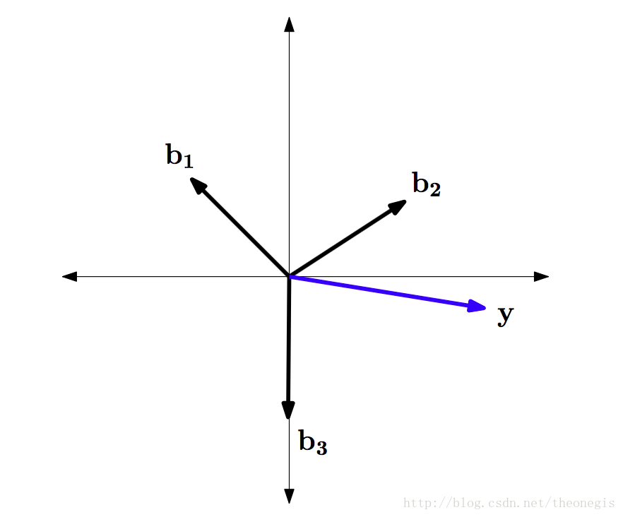
w = \mathrm{A}^{\mathrm{T}} \cdot y = \begin{bmatrix}-0.707 & 0.707 \\ 0.8 & 0.6 \\ 0 & -1\end{bmatrix} \cdot \begin{bmatrix}1.65 \\ -0.25\end{bmatrix} = \begin{bmatrix}-1.34 \\ 1.17 \\ 0.25\end{bmatrix} 原子和
y的几何意义如图1:
计算残差
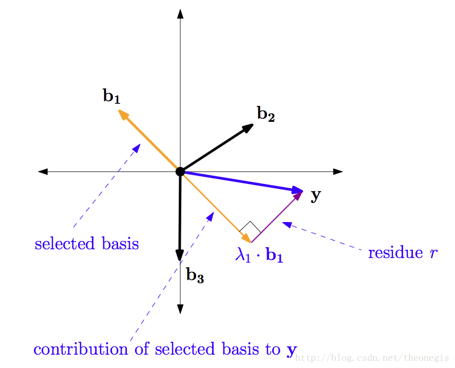
现在已经选定了第一个基
b_1 = \begin{bmatrix}-0.707 \\ 0.707\end{bmatrix} ,贡献值系数为
\lambda_1 = -1.34. 将该部分贡献值从
y中减去,残差为
r = y - \lambda_1 \cdot b_1 = \begin{bmatrix}1.65 \\ -0.25\end{bmatrix} - (-1.34) \cdot \begin{bmatrix}-0.707 \\ 0.707\end{bmatrix} = \begin{bmatrix}0.7 \\ 0.7\end{bmatrix}残差的几何意义如图2:
重复迭代
经过第一次迭代,我们选择出了基
b_1. 将选择出的基加入新的矩阵
\mathrm{A}_{new},即:
\mathrm{A}_{new} = [b_1] = \begin{bmatrix}-0.707 \\ 0.707\end{bmatrix}贡献系数矩阵可以写成
x_{rec} = \begin{bmatrix}-1.34 \\ 0 \\ 0\end{bmatrix}第一个元素是第一个贡献值-1.34,对应着第一个第一个基
b_1.
残差值为
r = \begin{bmatrix}0.7 \\ 0.7\end{bmatrix}现在需要从剩下的基
b_2和
b_3中选择对残差
r贡献最大的.
w = \begin{bmatrix}b_2 \\ b_3\end{bmatrix}^{\mathrm{T}} \cdot r = \begin{bmatrix}0.98 \\ -0.7\end{bmatrix}所以,
b_2的贡献值更大一些是0.98.
我们将选择的基
b_2添加到
\mathrm{A}_{new}得到
\mathrm{A}_{new} = \begin{bmatrix}b_1 & b_2\end{bmatrix} = \begin{bmatrix}-0.707 & 0.8 \\ 0.707 & 0.6\end{bmatrix}接下来的步骤和MP算法稍微有些不同. 这里,我们需要计算
\mathrm{A}_{new}对
y的贡献(而不是
b_2对
r的贡献)
我们使用最小二乘法(Least Square Problem)解决该该贡献值问题:
如何求得
\lambda_1和
\lambda_2的值使得
\lambda_1 \cdot \begin{bmatrix}-0.707 \\ 0.707\end{bmatrix} + \lambda_2 \cdot \begin{bmatrix}0.8 \\ 0.6\end{bmatrix}最接近
y = \begin{bmatrix}1.65 \\ -0.25\end{bmatrix}?
表示成数学语言为:
\min \|\mathrm{A}_{new} \cdot \mathbf{\lambda} - y\|_2在这个例子中,即
\min \|\begin{bmatrix}b_1 & b_2\end{bmatrix} = \begin{bmatrix}-0.707 & 0.8 \\ 0.707 & 0.6\end{bmatrix} \cdot \begin{bmatrix}\lambda_1 \\ \lambda_2\end{bmatrix} - \begin{bmatrix}1.65 \\ -0.25\end{bmatrix}\|_2对于
\min \|\mathrm{A}_{new} \cdot \mathbf{\lambda} - y\|_2的解可以直接使用公式:
\mathbf{\lambda} = \mathrm{A}_{new}^+ \cdot y其中,
\mathrm{A}_{new}^+是
\mathrm{A}_{new}的谓逆,
\mathrm{A}_{new}^+ = (\mathrm{A}_{new}^{\mathrm{T}} \cdot \mathrm{A}_{new})^{-1} \cdot \mathrm{A}_{new}^{\mathrm{T}}(注:可参看我的博文《Moore-Penrose广义逆矩阵》和《矛盾方程的最小二乘解法》)
在我们的例子中
\mathrm{A_{new}^+} = \begin{bmatrix}-0.707 & 0.8 \\ 0.707 & 0.6\end{bmatrix}^+ = \begin{bmatrix}-0.6062 & 0.8082 \\ 0.7143 & 0.7143\end{bmatrix}可以使用MATLAB中的内置函数pinv()进行伪逆的计算.
得到
\mathrm{A_{new}^+}后,可以计算
\mathbf{\lambda}\mathbf{\lambda} = \mathrm{A}_{new}^+ \cdot y = \begin{bmatrix}-0.6062 & 0.8082 \\ 0.7143 & 0.7143\end{bmatrix} \cdot \begin{bmatrix}1.65 \\ -0.25\end{bmatrix} = \begin{bmatrix}-1.2 \\ 1\end{bmatrix}得到
\mathbf{\lambda}以后,更新系数矩阵
x_{rec}为
x_{rec} = \begin{bmatrix}-1.2 \\ 1 \\ 0\end{bmatrix}同样的,
\mathbf{\lambda}在
x_{rec}第一个元素和第二个元素对应着选择出来的第一个和第二个基.
得到
\mathrm{A}_{new}和
\mathbf{\lambda}以后,我们可以计算残差
r = y - \mathrm{A}_{new} \cdot \mathbf{\lambda} = \begin{bmatrix}1.65 \\ -0.25\end{bmatrix} - \begin{bmatrix}-0.707 & 0.8 \\ 0.707 & 0.6\end{bmatrix} \cdot \begin{bmatrix}—1.2 \\ 1\end{bmatrix} = \begin{bmatrix}0 \\ 0\end{bmatrix}此时,残差值为
\begin{bmatrix}0 \\ 0\end{bmatrix},我们可以停止计算或者继续下一步计算(这里停止,可以节省一些计算工作).
最后一次迭代
这一步不是必须的,因为残差已经完全消除了(很多实现OMP的软件都需要输入稀疏度
K参数,这样经过
K次迭代以后,无论残差大小都会停止迭代).
重新组织信号系数
x_{rec} = \begin{bmatrix}-1.2 \\ 1 \\ 0\end{bmatrix},这刚好是原始的系数.
其他例子
给定
x = \begin{bmatrix}0 \\ 3 \\ 1 \\ 2\end{bmatrix}和
\mathrm{A} = \begin{bmatrix}-0.8 & 0.3 & 1 & 0.4 \\ -0.2 & 0.4 & -0.3 & -0.4 \\ 0.2 & 1 & -0.1 & 0.8 \end{bmatrix},
求得
y = \mathrm{A} \cdot x = \begin{bmatrix}2.7 \\ 0.1 \\ 4.5\end{bmatrix}现在给定
\mathrm{A}和
y,使用OMP算法求解
x.
- 我们有4个基(原子):
b_1 = \begin{bmatrix}-0.8 \\ -0.2 \\ 0.2\end{bmatrix} \qquad b_2 = \begin{bmatrix}0.3 \\ 0.4 \\ 1\end{bmatrix} \qquad b_3 = \begin{bmatrix}1 \\ -0.3 \\ -0.1\end{bmatrix} \qquad b_4 = \begin{bmatrix}0.4 \\ -0.4 \\ 0.8\end{bmatrix} \qquad- 由于基向量的长度不是1,所以我们首先进行标准化.
\hat{b_1} = b_1 / \|b_1\| = \begin{bmatrix}-0.8 \\ -0.2 \\ 0.2\end{bmatrix} / \sqrt{(-0.8)^2 + (-0.4)^2 + (0.2)^2} = \begin{bmatrix}-0.9428 \\ -0.2357 \\ 0.2357\end{bmatrix}\hat{b_2} = b_2 / \|b_2\| = \begin{bmatrix}0.2680 \\ 0.3578 \\ 0.8940\end{bmatrix}\hat{b_3} = b_3 / \|b_3\| = \begin{bmatrix}0.9535 \\ -0.2860 \\ 0.0953\end{bmatrix}\hat{b_2} = b_2 / \|b_2\| = \begin{bmatrix}0.4082 \\ -0.4082 \\ -0.8165\end{bmatrix}- 标准化的基向量对
y的贡献
ww = \hat{\mathrm{A}}^{\mathrm{T}} \cdot y = \begin{bmatrix}-0.9428 & 0.2680 & 0.9535 & 0.4082 \\ -0.2357 & 0.3578 & -0.2860 & -0.4082\\ 0.2357 & 0.9840 & -0.0953 & -0.8165\end{bmatrix}^{\mathrm{T}} \cdot \begin{bmatrix}2.7 \\ 0.1 \\ 4.5\end{bmatrix} = \begin{bmatrix}-1.5085 \\ 4.7852 \\ 2.1167 \\ 4.7357\end{bmatrix}- 第二个基向量
b_2贡献值最大,所以将
b_2加入到
\mathrm{A}_{new}\mathrm{A}_{new} = b_2 = \begin{bmatrix}0.3 \\ 0.4 \\ 1\end{bmatrix}- 利用最小二乘法计算
x_{rec}L_p = \mathrm{A}_{new}^+ \cdot y = [4.28]
因为
L_p对应着第二个基向量,所以
x_{rec} = \begin{bmatrix}0 \\ 4.28 \\ 0 \\ 0\end{bmatrix}- 接下来计算残差
r = y - \mathrm{A}_{new} \cdot L_p = \begin{bmatrix}2.7 \\ 0.1 \\ 4.5\end{bmatrix} - \begin{bmatrix}0.3 \\ 0.4 \\ 1\end{bmatrix} \cdot 4.28 = \begin{bmatrix}1.416 \\ -1.612 \\ 0.22\end{bmatrix}- 接下来重复第3步,计算
\hat{b_1},
\hat{b_1}和
\hat{b_1}对
r的贡献.
w = \hat{\mathrm{A}}^{\mathrm{T}} \cdot r = \begin{bmatrix}-0.9428 & 0.9535 & 0.4082 \\ -0.2357 & -0.2860 & -0.4082\\ 0.2357 & -0.0953 & -0.8165\end{bmatrix}^{\mathrm{T}} \cdot \begin{bmatrix}1.416 \\ -1.612 \\ 0.22\end{bmatrix} = \begin{bmatrix}-0.9032 \\ 1.7902 \\ 1.4158\end{bmatrix}
选择第二个贡献最大的基
b_3,其贡献值为1.7902.
- 将选择的
b_3加入到
\mathrm{A}_{new}中
\mathrm{A}_{new} = \begin{bmatrix}b_1 & b_2\end{bmatrix} = \begin{bmatrix}0.3 & 1\\ 0.4 & -0.3\\ 1 & -0.1\end{bmatrix}- 用最小二乘法计算
L_p = \mathrm{A}_{new}^+ \cdot y = \begin{bmatrix}4.1702 \\ 1.7149\end{bmatrix}
这个
L_p对应着
b_2和
b_3,因此
x_{rec} = \begin{bmatrix}0 \\ 4.172 \\ 1.7149 \\ 0\end{bmatrix}- 接着计算残差
r = y - \mathrm{A}_{new} \cdot L_p = \begin{bmatrix}2.7 \\ 0.1 \\ 4.5\end{bmatrix} - \begin{bmatrix}0.3 & 1\\ 0.4 & -0.3\\ 1 & -0.1\end{bmatrix} \cdot \begin{bmatrix}4.172 \\ 1.7149\end{bmatrix} = \begin{bmatrix}-0.266 \\ -1.0536 \\ 0.5012\end{bmatrix}- 重复步骤2,进行最后一次迭代
- 计算
b_1和
b_4的贡献值
w = \begin{bmatrix}\hat{b_1} & \hat{b_2}\end{bmatrix} \cdot r = \begin{bmatrix}-0.9428 & 0.4082 \\ -0.2357 & -0.4082\\ 0.2357 & -0.8165\end{bmatrix}^{\mathrm{T}} \cdot \begin{bmatrix}-0.266 \\ -1.0536 \\ 0.5012\end{bmatrix} = \begin{bmatrix}0.6172 \\ 0.7308\end{bmatrix}
这里
b_4提供了最大贡献值0.7308.
- 将
b_4加入
\mathrm{A}_{new} = \begin{bmatrix}0.3 & 1 & 0.4 \\ 0.4 & -0.3 & -0.4 \\ 1 & -0.1 & 0.8\end{bmatrix}- 利用最小二乘计算
L_p = \mathrm{A}_{new}^+ \cdot y = \begin{bmatrix}3 \\ 2 \\1\end{bmatrix},对应的
x_{rec} = \begin{bmatrix}0 \\ 3 \\ 1 \\ 2\end{bmatrix}- 接着计算残差
r = y - \mathrm{A}_{new} \cdot L_p = \begin{bmatrix}2.7 \\ 0.1 \\ 4.5\end{bmatrix} - \begin{bmatrix}0.3 & 1 & 0.4\\ 0.4 & -0.3 & -0.4\\ 1 & -0.1 & 0.8\end{bmatrix} \cdot \begin{bmatrix}3 \\ 1 \\ 2\end{bmatrix} = \begin{bmatrix}0 \\ 0 \\ 0\end{bmatrix}- 我们的迭代到此为止,因为此时残差已经为0,重建的
x为
x_{rec} = \begin{bmatrix}0 \\ 3 \\1 \\2\end{bmatrix},和原来的信号相同.
需要注意的问题
通过上面的迭代计算过程,我们应该注意如下几点:
- OMP中最大贡献值的计算需要对基向量进行标准化处理,不是由原始基得到的.
- 如果给定的基向量已经是单位向量,则不需要进行标准化.
- 基向量对
y值的贡献的计算是通过标准化以后的基向量和残差的点积进行计算的.
- 在MP算法中,重建系数
x_{rec}的计算是通过基向量和残差的点积进行计算的,在OMP算法中,
x_{rec}的计算是通过最小二乘法得到
\mathrm{A}_{new}相对于
y的系数得到的,即
L_p的计算.
L_p向量中的值直接对应于
x_{rec}的相应位置.
\mathrm{A}_{new}通过每次对基向量的选择得到. 这个过程是需要时间的,因此OMP比MP慢. (不是应该OMP收敛的快吗?)
- 残差
r的计算通过原始的
y值和
\mathrm{A}_{new},
L_p得到.
- 迭代的次数最多等于
\mathrm{A}矩阵的行数M,或者如果给定了稀疏度
K,则迭代
K次. 如果
K < M,则已知的
K可以加快计算结束,如果
K未知,则迭代
M次.
说明总结
在正交匹配追踪OMP中,残差总是与已经选择过的原子正交的。这意味着一个原子不会被选择两次,结果会在有限的几步收敛。
OMP算法 步骤描述:
输入:字典矩阵
\mathrm{A},采样向量
y,稀疏度
k.
输出:
x的
K稀疏逼近
\hat{x}.
初始化:残差
r_0 = y,索引集
\Lambda_0 = \emptyset,
t=1.
循环执行步骤1-5:
- 找出残差
r和字典矩阵的列
\mathrm{A}_i积中最大值所对应的脚标
\lambda,即
\lambda_t = \arg \max_{i=1,\cdots, N}\left|<r_{t-1},\mathrm{A}_i>\right|.
- 更新索引集
\Lambda_t = \Lambda_{t-1} \cup \{\lambda_t\},记录找到的字典矩阵中的重建原子集合
A_t = [A_{t-1}, A_{\lambda_t}].
- 由最小二乘得到
\hat{x}_t = \arg \min \left|| y - A_t \hat{x} |\right|.
- 更新残差
r_t = y - A_t \hat{x}_t,
t=t+1.
- 判断是否满足
t > K,若满足,则迭代停止;若不满足,则继续执行步骤1.